COUNTIF and COUNTIFS in Google Sheets
Learn how to use COUNTIF and COUNTIFS in Google Sheets to count cells by condition. Covers comparison operators, wildcards, and multiple criteria examples.
Sheets Bootcamp
February 26, 2026
COUNTIF in Google Sheets counts how many cells in a range match a condition you specify. It is one of the most used counting functions in the IF Statements family and works with text, numbers, and comparison operators. This guide covers COUNTIF syntax, step-by-step examples, wildcard matching, and how to upgrade to COUNTIFS when you need multiple criteria.
In This Guide
- What Is COUNTIF?
- COUNTIF Syntax
- How to Use COUNTIF: Step-by-Step
- COUNTIF with Comparison Operators
- COUNTIF with Wildcards
- COUNTIFS Syntax (Multiple Criteria)
- How to Use COUNTIFS: Step-by-Step
- COUNTIFS Example: Count by Salesperson and Region
- Common Mistakes
- Tips
- FAQ
What Is COUNTIF?
COUNTIF counts the number of cells in a range that meet a single condition. You tell it where to look and what to look for, and it returns a count.
Use COUNTIF when you need to answer questions like “how many sales came from Diagon Alley?” or “how many orders had revenue above $400?” If you need to add up values instead of counting them, SUMIF is the function you want.
COUNTIF Syntax
=COUNTIF(range, criterion)| Parameter | Description | Required |
|---|---|---|
| range | The range of cells to evaluate | Yes |
| criterion | The condition that determines which cells to count. Can be a number, text, expression, or cell reference. | Yes |
When using comparison operators like greater than or less than, wrap the entire criterion in quotes. Write ">400", not >400. Google Sheets treats the criterion as text, so the operator and value must be a single quoted string.
How to Use COUNTIF: Step-by-Step
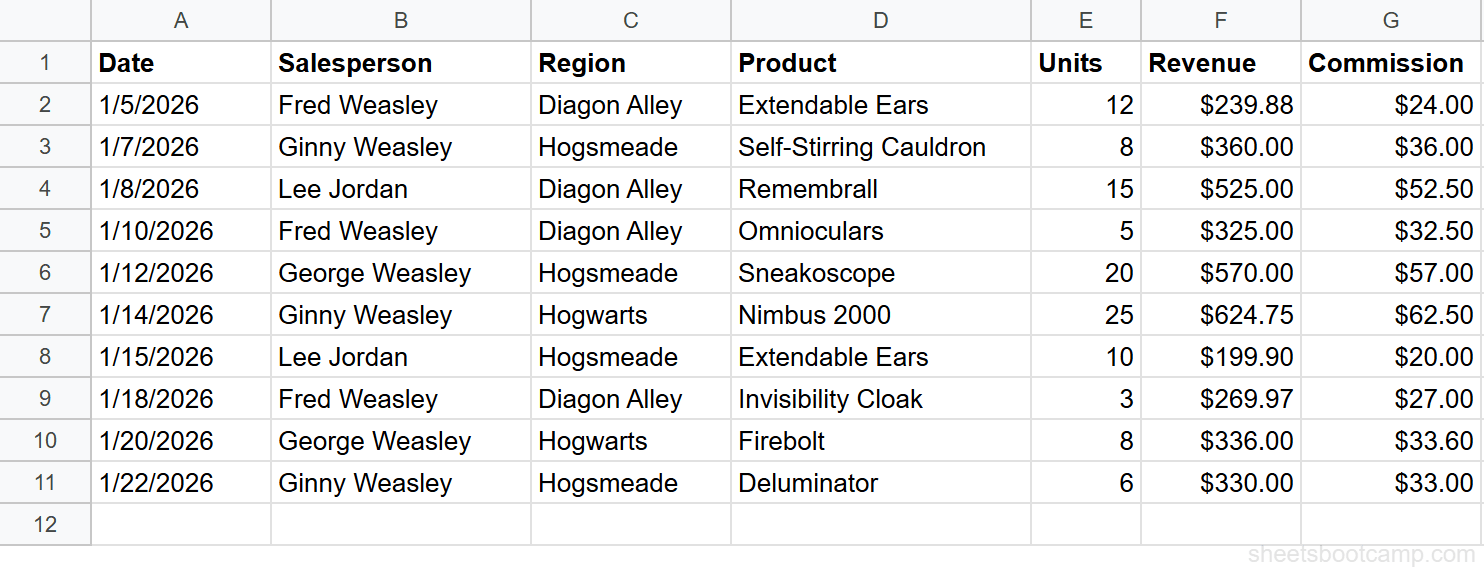
We’ll use a sales records table with 10 transactions. The goal: count how many sales happened in the Diagon Alley region.
Review your sales data
Your spreadsheet has sales records in columns A through G. Each row contains a Date, Salesperson, Region, Product, Units, Revenue, and Commission.
| A | B | C | D | E | F | G | |
|---|---|---|---|---|---|---|---|
| 1 | Date | Salesperson | Region | Product | Units | Revenue | Commission |
| 2 | 1/5/2026 | Fred Weasley | Diagon Alley | Extendable Ears | 12 | $239.88 | $24.00 |
| 3 | 1/7/2026 | Ginny Weasley | Hogsmeade | Self-Stirring Cauldron | 8 | $360.00 | $36.00 |
| 4 | 1/8/2026 | Lee Jordan | Diagon Alley | Remembrall | 15 | $525.00 | $52.50 |
| 5 | 1/10/2026 | Fred Weasley | Diagon Alley | Omnioculars | 5 | $325.00 | $32.50 |
| 6 | 1/12/2026 | George Weasley | Hogsmeade | Sneakoscope | 20 | $570.00 | $57.00 |
| 7 | 1/14/2026 | Ginny Weasley | Hogwarts | Nimbus 2000 | 25 | $624.75 | $62.50 |
| 8 | 1/15/2026 | Lee Jordan | Hogsmeade | Extendable Ears | 10 | $199.90 | $20.00 |
| 9 | 1/18/2026 | Fred Weasley | Diagon Alley | Invisibility Cloak | 3 | $269.97 | $27.00 |
| 10 | 1/20/2026 | George Weasley | Hogwarts | Firebolt | 8 | $336.00 | $33.60 |
| 11 | 1/22/2026 | Ginny Weasley | Hogsmeade | Deluminator | 6 | $330.00 | $33.00 |
Enter the COUNTIF formula
Select cell I2. Enter this formula to count sales in Diagon Alley:
=COUNTIF(C2:C11, "Diagon Alley")Here is what each part does:
C2:C11— the Region column, rows 2 through 11"Diagon Alley"— the text to match (case-insensitive)
Check the result
Press Enter. The formula returns 4. Four rows in the Region column contain “Diagon Alley”: rows 2, 4, 5, and 9.
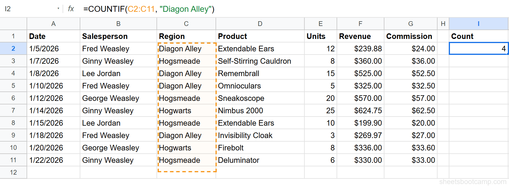
COUNTIF is case-insensitive. "Diagon Alley", "diagon alley", and "DIAGON ALLEY" all match the same cells.
COUNTIF with Comparison Operators
COUNTIF works with comparison operators to count cells above or below a threshold. You can use >, <, >=, <=, <> (not equal to), and =.
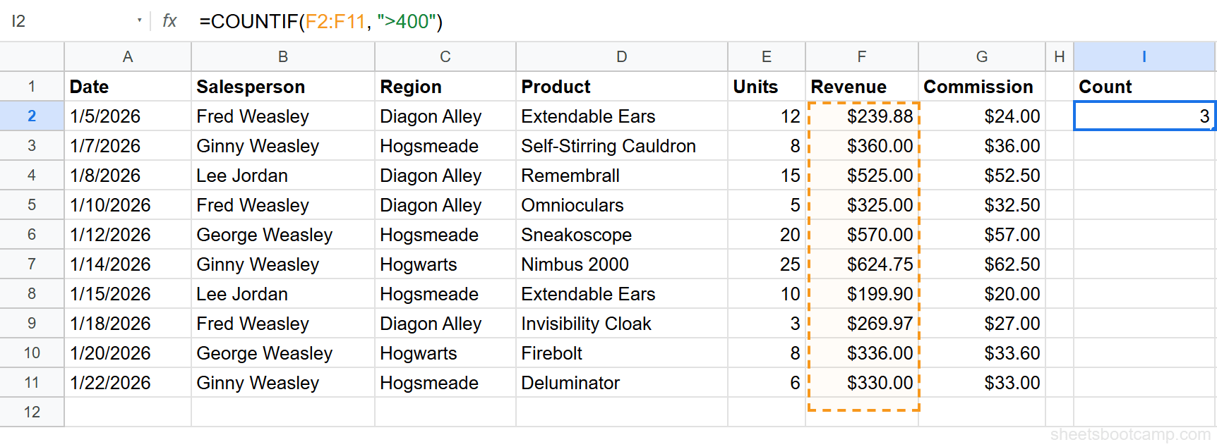
To count how many sales had revenue greater than $400:
=COUNTIF(F2:F11, ">400")This returns 3. Three transactions exceeded $400 in revenue: $525.00 (row 4), $570.00 (row 6), and $624.75 (row 7).
To make the threshold dynamic, reference a cell instead of hardcoding the number:
=COUNTIF(F2:F11, ">"&I1)Place your threshold value in I1, and the formula adjusts automatically when you change it.
COUNTIF with Wildcards
COUNTIF supports two wildcard characters for pattern matching:
*(asterisk) — matches any number of characters?(question mark) — matches exactly one character
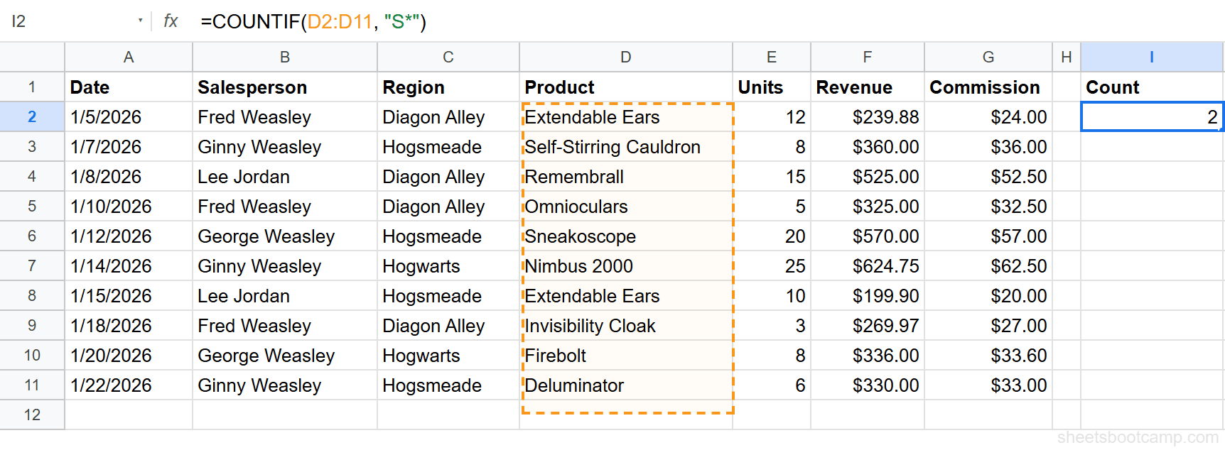
To count products that start with the letter “S”:
=COUNTIF(D2:D11, "S*")This returns 2. Two products start with “S”: Self-Stirring Cauldron (row 3) and Sneakoscope (row 6).
To count how many times a specific product appears, use an exact text match:
=COUNTIF(D2:D11, "Extendable Ears")This returns 2. Extendable Ears appears in rows 2 and 8.
Use "*"&A1&"*" to count cells containing the value in A1 anywhere in the text. This is how you build a “count if cell contains” formula with a dynamic reference.
COUNTIFS Syntax (Multiple Criteria)
COUNTIFS counts cells that meet two or more conditions at the same time. Each condition has its own range and criterion, and all conditions must be true for a cell to be counted.
=COUNTIFS(criteria_range1, criterion1, criteria_range2, criterion2, ...)| Parameter | Description | Required |
|---|---|---|
| criteria_range1 | The first range to evaluate | Yes |
| criterion1 | The condition for the first range | Yes |
| criteria_range2 | The second range to evaluate | Yes |
| criterion2 | The condition for the second range | Yes |
| … | Additional range/criterion pairs | No |
COUNTIFS uses AND logic. A row is only counted when every condition is met. If you need OR logic (count rows matching condition A or condition B), add separate COUNTIF calls together instead.
How to Use COUNTIFS: Step-by-Step
We’ll count sales in Diagon Alley where revenue exceeded $300. This requires two conditions: the Region must be “Diagon Alley” and the Revenue must be greater than $300.
Enter this formula in cell I2:
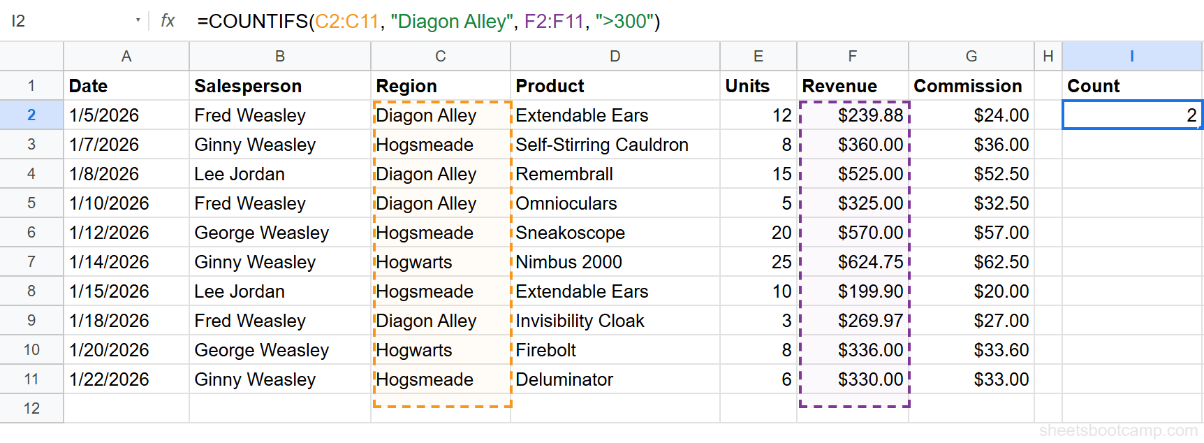
=COUNTIFS(C2:C11, "Diagon Alley", F2:F11, ">300")Here is what each part does:
C2:C11, "Diagon Alley"— first condition: Region is Diagon AlleyF2:F11, ">300"— second condition: Revenue exceeds $300
The formula returns 2. Two Diagon Alley sales had revenue above $300:
| Row | Region | Revenue | Counted? |
|---|---|---|---|
| 2 | Diagon Alley | $239.88 | No (revenue under $300) |
| 4 | Diagon Alley | $525.00 | Yes |
| 5 | Diagon Alley | $325.00 | Yes |
| 9 | Diagon Alley | $269.97 | No (revenue under $300) |
Every range in COUNTIFS must have the same number of rows. C2:C11 has 10 rows, so F2:F11 must also have 10 rows. Mismatched ranges cause a #VALUE! error.
COUNTIFS Example: Count by Salesperson and Region
Count how many sales Fred Weasley made in Diagon Alley:
=COUNTIFS(B2:B11, "Fred Weasley", C2:C11, "Diagon Alley")This returns 3. Fred Weasley has three Diagon Alley transactions: Extendable Ears (row 2), Omnioculars (row 5), and Invisibility Cloak (row 9).
You can add a third condition. To count Fred Weasley’s Diagon Alley sales where revenue exceeded $250:
=COUNTIFS(B2:B11, "Fred Weasley", C2:C11, "Diagon Alley", F2:F11, ">250")This returns 2. The Omnioculars sale ($325.00) and Invisibility Cloak sale ($269.97) both qualify. The Extendable Ears sale ($239.88) falls short.
Common Mistakes
Forgetting quotes around comparison operators
This breaks:
=COUNTIF(F2:F11, >400)This works:
=COUNTIF(F2:F11, ">400")The operator and value must be wrapped together in a single string. Without quotes, Google Sheets cannot parse the criterion.
Counting formatted numbers as text
If your Revenue column stores values as text (like “$400” typed manually instead of formatted as currency), COUNTIF’s numeric comparison won’t work. The cells look like numbers but are actually text strings. Select the range and check the format under Format > Number. True numbers align to the right by default. Text masquerading as numbers aligns to the left.
Mismatched range sizes in COUNTIFS
Every criteria_range in COUNTIFS must contain the same number of rows. If your first range is C2:C11 (10 rows) and your second range is F2:F15 (14 rows), you get a #VALUE! error. Double-check that all ranges start and end at the same rows.
Tips
1. Combine COUNTIF with conditional formatting to spot duplicates. Use =COUNTIF(A:A, A1) > 1 as a conditional formatting custom formula to highlight any value that appears more than once in column A.
2. Reference cells instead of hardcoding criteria. Write =COUNTIF(C2:C11, I1) and place “Diagon Alley” in I1. When you change I1, the count updates. This is more useful than editing the formula each time.
3. Use COUNTIFS for date ranges. Count transactions between two dates with =COUNTIFS(A2:A11, ">="&DATE(2026,1,10), A2:A11, "<="&DATE(2026,1,20)). COUNTIFS handles the AND logic to count only dates within the window.
COUNTIF and COUNTIFS follow the same AND/OR patterns as IF with AND and OR. If COUNTIFS handles AND logic natively, use addition for OR: =COUNTIF(C2:C11, "Diagon Alley") + COUNTIF(C2:C11, "Hogwarts") counts cells matching either region.
Related Google Sheets Tutorials
- IF Statements in Google Sheets — the parent guide covering IF, nested IF, and conditional logic
- SUMIF and SUMIFS in Google Sheets — add up values by condition instead of counting them
- Conditional Formatting in Google Sheets — highlight cells visually based on rules
- AND and OR Functions — combine multiple conditions inside IF formulas
Frequently Asked Questions
What is the difference between COUNTIF and COUNTIFS?
COUNTIF checks one condition against one range. COUNTIFS checks multiple conditions across multiple ranges. Use COUNTIF when you have a single criterion, and COUNTIFS when you need two or more conditions to be true at the same time.
How do I count cells that contain specific text in Google Sheets?
Use COUNTIF with a wildcard pattern. For example, =COUNTIF(D2:D11, "*ears*") counts every cell in D2:D11 that contains the word “ears” anywhere in the text. The asterisk (*) matches any number of characters.
Can COUNTIF count cells greater than a number?
Yes. Put the comparison operator and number inside quotes together. For example, =COUNTIF(F2:F11, ">400") counts every cell in F2:F11 with a value greater than 400.
How do I use COUNTIF with multiple criteria in one column?
Add separate COUNTIF calls together. For example, =COUNTIF(C2:C11, "Diagon Alley") + COUNTIF(C2:C11, "Hogwarts") counts cells matching either region. For AND logic across different columns, use COUNTIFS instead.