SUMIF and SUMIFS in Google Sheets
Learn how to use SUMIF and SUMIFS in Google Sheets to add values based on one or multiple conditions. Step-by-step examples, syntax, and common mistakes.
Sheets Bootcamp
February 27, 2026
SUMIF in Google Sheets adds values in a range based on a condition you specify. It belongs to the same family of conditional functions covered in our IF function guide, and once you need more than one condition, SUMIFS picks up where SUMIF leaves off. We’ll cover both functions, walk through real examples, and highlight the argument order difference that catches most people off guard.
In This Guide
- What Is SUMIF?
- SUMIF Syntax
- How to Use SUMIF: Step-by-Step
- SUMIF with Comparison Operators
- What Is SUMIFS?
- SUMIFS Syntax
- How to Use SUMIFS: Step-by-Step
- SUMIF vs SUMIFS: Key Differences
- Common Mistakes
- Tips
- Related Google Sheets Tutorials
- FAQ
What Is SUMIF?
SUMIF adds values in a range where a corresponding cell meets a condition. Use it when you want to total revenue by region, sum expenses by category, or add up hours by employee.
SUMIF Syntax
=SUMIF(range, criterion, [sum_range])| Parameter | Description | Required |
|---|---|---|
| range | The range of cells to evaluate against the criterion | Yes |
| criterion | The condition that determines which cells to include. Text, numbers, or expressions like ">400" | Yes |
| sum_range | The range of cells to add. If omitted, SUMIF adds the values in range instead | No |
SUMIF puts the criteria range first: =SUMIF(range, criterion, sum_range). This is the opposite of SUMIFS, which puts the sum range first. Mixing them up is the most common SUMIF mistake.
How to Use SUMIF: Step-by-Step
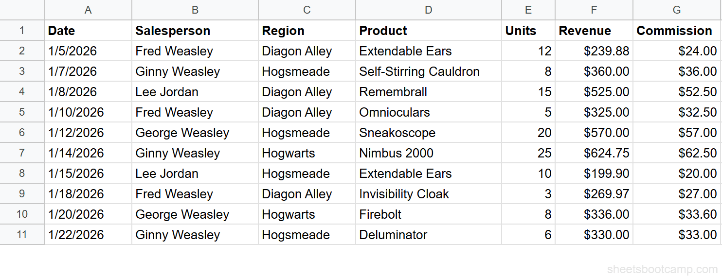
We’ll use a sales records table with 10 transactions. The goal: add up all revenue from the Baker Street region.
Review your data
Your spreadsheet has sales records in columns A through G. Each row contains a Date, Salesperson, Region, Product, Units, Revenue, and Commission.
| A | B | C | D | E | F | G | |
|---|---|---|---|---|---|---|---|
| 1 | Date | Salesperson | Region | Product | Units | Revenue | Commission |
| 2 | 1/5/2026 | Sherlock Holmes | Baker Street | Listening Device | 12 | $239.88 | $24.00 |
| 3 | 1/7/2026 | Irene Adler | Scotland Yard | Forensic Chemistry Set | 8 | $360.00 | $36.00 |
| 4 | 1/8/2026 | Inspector Lestrade | Baker Street | Pocket Watch | 15 | $525.00 | $52.50 |
| 5 | 1/10/2026 | Sherlock Holmes | Baker Street | Field Binoculars | 5 | $325.00 | $32.50 |
| 6 | 1/12/2026 | Mycroft Holmes | Scotland Yard | Cipher Decoder | 20 | $570.00 | $57.00 |
| 7 | 1/14/2026 | Irene Adler | Whitehall | Magnifying Glass | 25 | $624.75 | $62.50 |
| 8 | 1/15/2026 | Inspector Lestrade | Scotland Yard | Listening Device | 10 | $199.90 | $20.00 |
| 9 | 1/18/2026 | Sherlock Holmes | Baker Street | Disguise Kit | 3 | $269.97 | $27.00 |
| 10 | 1/20/2026 | Mycroft Holmes | Whitehall | Brass Telescope | 8 | $336.00 | $33.60 |
| 11 | 1/22/2026 | Irene Adler | Scotland Yard | Lockpick Set | 6 | $330.00 | $33.00 |
Enter the SUMIF formula
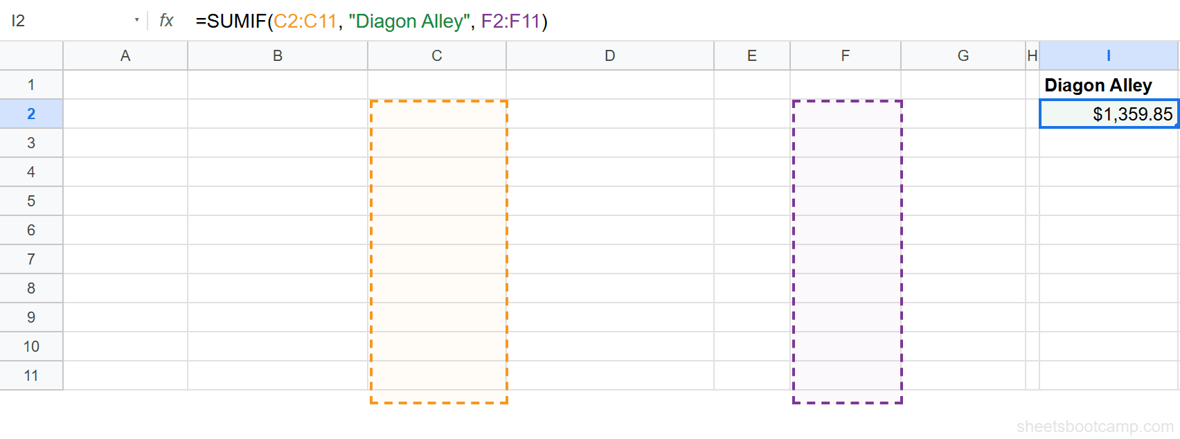
Select cell I2 and enter:
=SUMIF(C2:C11, "Baker Street", F2:F11)Here is what each part does:
C2:C11— the range to check (Region column)"Baker Street"— the criterion (match rows where Region equals Baker Street)F2:F11— the sum range (add the Revenue values for matching rows)
Check the result
Press Enter. The formula returns $1,359.85. That is the total revenue from the four Baker Street transactions: $239.88 + $525.00 + $325.00 + $269.97.
SUMIF is not case-sensitive. “Baker Street”, “baker street”, and “BAKER STREET” all match the same rows.
SUMIF with Comparison Operators
SUMIF works with more than exact text matches. You can use comparison operators to sum values above or below a threshold.
To add all revenue values greater than $400:
=SUMIF(F2:F11, ">400", F2:F11)This returns $1,719.75. Three transactions have revenue above $400: $525.00, $570.00, and $624.75.
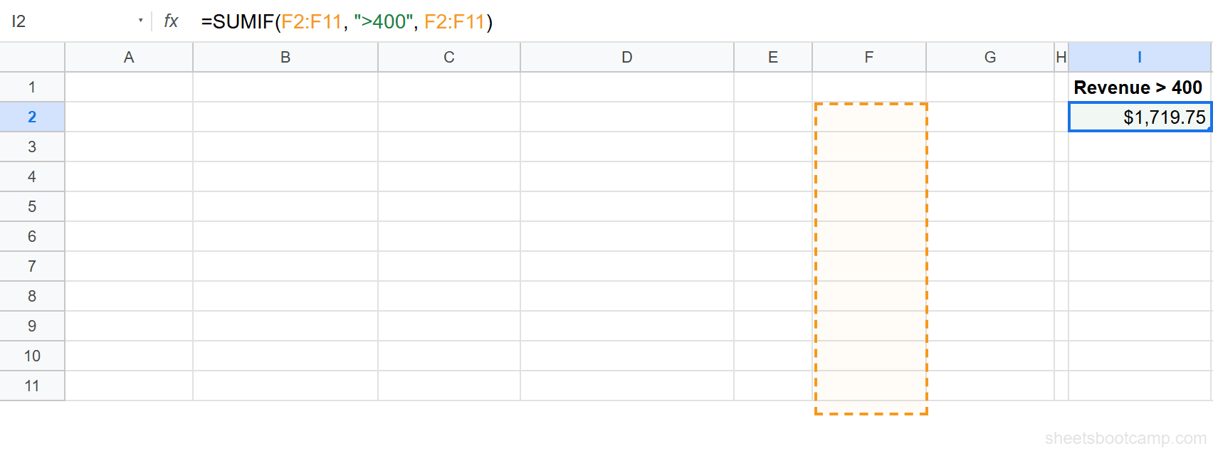
When the criteria range and sum range are the same column, you can omit the third argument. =SUMIF(F2:F11, ">400") returns the same $1,719.75 result.
Common comparison operators you can use as criteria:
| Operator | Meaning | Example Criterion |
|---|---|---|
> | Greater than | ">400" |
< | Less than | "<200" |
>= | Greater than or equal to | ">=500" |
<= | Less than or equal to | "<=300" |
<> | Not equal to | <>"Whitehall" |
What Is SUMIFS?
SUMIFS adds values based on two or more conditions. When you need to filter by region and salesperson at the same time, SUMIFS handles it in a single formula.
SUMIFS Syntax
=SUMIFS(sum_range, criteria_range1, criterion1, criteria_range2, criterion2, ...)| Parameter | Description | Required |
|---|---|---|
| sum_range | The range of cells to add | Yes |
| criteria_range1 | The first range to evaluate | Yes |
| criterion1 | The condition for criteria_range1 | Yes |
| criteria_range2 | The second range to evaluate | No |
| criterion2 | The condition for criteria_range2 | No |
You can add as many criteria_range/criterion pairs as you need.
SUMIFS puts the sum range FIRST. This is the opposite of SUMIF, where the criteria range comes first. Swapping the order is the number one SUMIFS mistake and returns wrong results without an error message.
How to Use SUMIFS: Step-by-Step
Using the same sales data, we want total revenue where the salesperson is Sherlock Holmes AND the region is Baker Street.
Enter the SUMIFS formula
Select cell I2 and enter:
=SUMIFS(F2:F11, B2:B11, "Sherlock Holmes", C2:C11, "Baker Street")Here is what each part does:
F2:F11— the sum range (Revenue column, listed first in SUMIFS)B2:B11— first criteria range (Salesperson column)"Sherlock Holmes"— first criterion (match Sherlock Holmes)C2:C11— second criteria range (Region column)"Baker Street"— second criterion (match Baker Street)

Check the result
Press Enter. The formula returns $834.85. Sherlock Holmes has three Baker Street transactions: $239.88 + $325.00 + $269.97.
You can also combine text criteria with comparison operators. For example, to sum revenue in Baker Street where revenue exceeds $300:
=SUMIFS(F2:F11, C2:C11, "Baker Street", F2:F11, ">300")This returns $850.00 ($525.00 + $325.00). Only two Baker Street transactions have revenue above $300.
SUMIF vs SUMIFS: Key Differences
| Feature | SUMIF | SUMIFS |
|---|---|---|
| Number of conditions | One | Two or more |
| Argument order | Criteria range first, then sum range | Sum range first, then criteria pairs |
| Syntax | =SUMIF(range, criterion, sum_range) | =SUMIFS(sum_range, range1, criterion1, ...) |
| Comparison operators | Yes | Yes |
| Wildcards (* and ?) | Yes | Yes |
The argument order is the biggest difference. Writing SUMIFS with the SUMIF argument order (or vice versa) is a silent error. Google Sheets will not warn you. It will return a wrong number.
Common Mistakes
Swapping argument order between SUMIF and SUMIFS
SUMIF: criteria range first. SUMIFS: sum range first. If you write =SUMIFS(C2:C11, "Baker Street", F2:F11) with the SUMIF argument order, Google Sheets tries to sum the Region column, which contains text, and returns 0. No error appears, which makes this hard to catch.
Forgetting quotes around comparison operators
Comparison operators need to be inside double quotes. =SUMIF(F2:F11, >400, F2:F11) breaks because >400 is not a valid expression. Write ">400" with the quotes.
Mismatched range sizes in SUMIFS
Every criteria range and the sum range must be the same size. If your sum range is F2:F11 (10 rows) but a criteria range is C2:C8 (7 rows), SUMIFS returns a #VALUE! error. Keep all ranges the same length.
Tips
1. Use SUMIFS even for a single condition. SUMIFS works with one criteria pair too, and it keeps your formulas consistent. You won’t have to remember which argument order to use if you standardize on SUMIFS.
2. Reference cells for criteria. Instead of hardcoding "Baker Street", reference a cell: =SUMIF(C2:C11, I1, F2:F11). This lets you change the filter value without editing the formula.
3. Combine SUMIF with COUNTIF for averages. To get the average revenue per transaction for a region, divide SUMIF by COUNTIF: =SUMIF(C2:C11, "Baker Street", F2:F11) / COUNTIF(C2:C11, "Baker Street"). This returns $339.96, the average of the four Baker Street sales.
For more flexible summarization with grouping and filtering, try QUERY with GROUP BY. QUERY can produce summary tables with multiple aggregations in a single formula.
Related Google Sheets Tutorials
- IF Function: The Complete Guide — covers IF, nested IF, and logical conditions
- COUNTIF and COUNTIFS in Google Sheets — count cells that match conditions instead of summing them
- QUERY Function Guide — filter, group, and aggregate data with SQL-like syntax
- IF with AND / OR — combine multiple conditions in IF statements, similar logic to SUMIFS
Frequently Asked Questions
What is the difference between SUMIF and SUMIFS?
SUMIF adds values based on a single condition. SUMIFS adds values based on two or more conditions. They also use different argument orders: SUMIF takes the criteria range first, while SUMIFS takes the sum range first.
Why is the argument order different in SUMIF vs SUMIFS?
SUMIF was designed first with the syntax =SUMIF(range, criterion, sum_range). When Google added SUMIFS for multiple criteria, the sum_range moved to the front so that additional criteria_range/criterion pairs could be appended without limit. The result is two functions with reversed argument orders.
Can SUMIF add values greater than a number?
Yes. Use a comparison operator inside quotes as the criterion. For example, =SUMIF(F2:F11, ">400", F2:F11) adds all values in the range that are greater than 400.
How do you use SUMIF with multiple criteria in Google Sheets?
Use SUMIFS instead of SUMIF. SUMIFS accepts multiple criteria_range/criterion pairs. For example, =SUMIFS(F2:F11, B2:B11, "Sherlock Holmes", C2:C11, "Baker Street") adds revenue where the salesperson is Sherlock Holmes and the region is Baker Street.