Nested IF in Google Sheets (with Examples)
Learn how to write nested IF statements in Google Sheets. Covers multi-tier classification, letter grades, tiered commission, and when to switch to IFS.
Sheets Bootcamp
February 23, 2026
A nested IF in Google Sheets places one IF function inside another to handle more than two outcomes. When a single TRUE/FALSE split is not enough, nesting lets you test additional conditions in sequence, returning a different result for each.
This guide walks through three practical examples using real sales data: a 3-tier revenue classification, 4-tier letter grades, and a tiered commission calculation. We also cover the mistakes that trip people up and when to stop nesting altogether.
In This Guide
- How Nested IF Works
- Step-by-Step: Classify Revenue as High, Medium, or Low
- Example: 4-Tier Letter Grades
- Example: Tiered Commission Rates
- Common Mistakes
- When to Stop Nesting
- Tips for Readable Nested IFs
- Related Google Sheets Tutorials
- FAQ
How Nested IF Works
A standard IF function handles two outcomes: one for TRUE, one for FALSE. A nested IF replaces the FALSE branch with another IF, adding a third outcome. Each additional nest adds one more possible result.
Here is the structure for three outcomes:
=IF(condition1, result1, IF(condition2, result2, default))Google Sheets reads this left to right. It checks condition1 first. If TRUE, it returns result1 and stops. If FALSE, it moves to the inner IF and checks condition2. If that is TRUE, it returns result2. If both conditions are FALSE, it returns default.
The key detail: order matters. Google Sheets stops at the first TRUE condition. If you check for “greater than 300” before “greater than 500,” every value above 300 matches the first condition, and the 500 threshold never gets tested.
Always test the most restrictive condition first. In a nested IF that classifies values into ranges, start with the highest threshold and work down.
Step-by-Step: Classify Revenue as High, Medium, or Low
We’ll use a sales records table with 10 rows of data. The goal: add a column H that labels each sale’s revenue as “High” (>=$500), “Medium” ($300-$499), or “Low” (under $300).
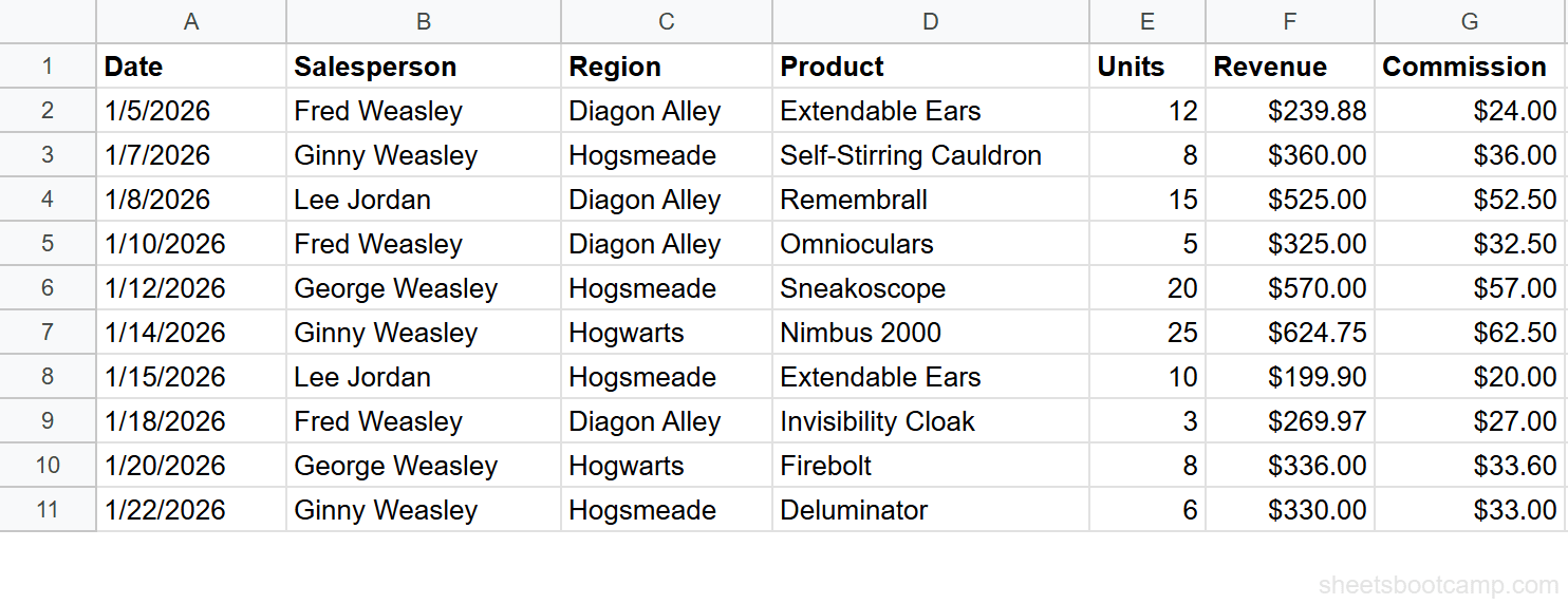
Review the data
The sales data has 7 columns: Date, Salesperson, Region, Product, Units, Revenue, and Commission. Column F (Revenue) contains the values we want to classify.
Enter the nested IF formula
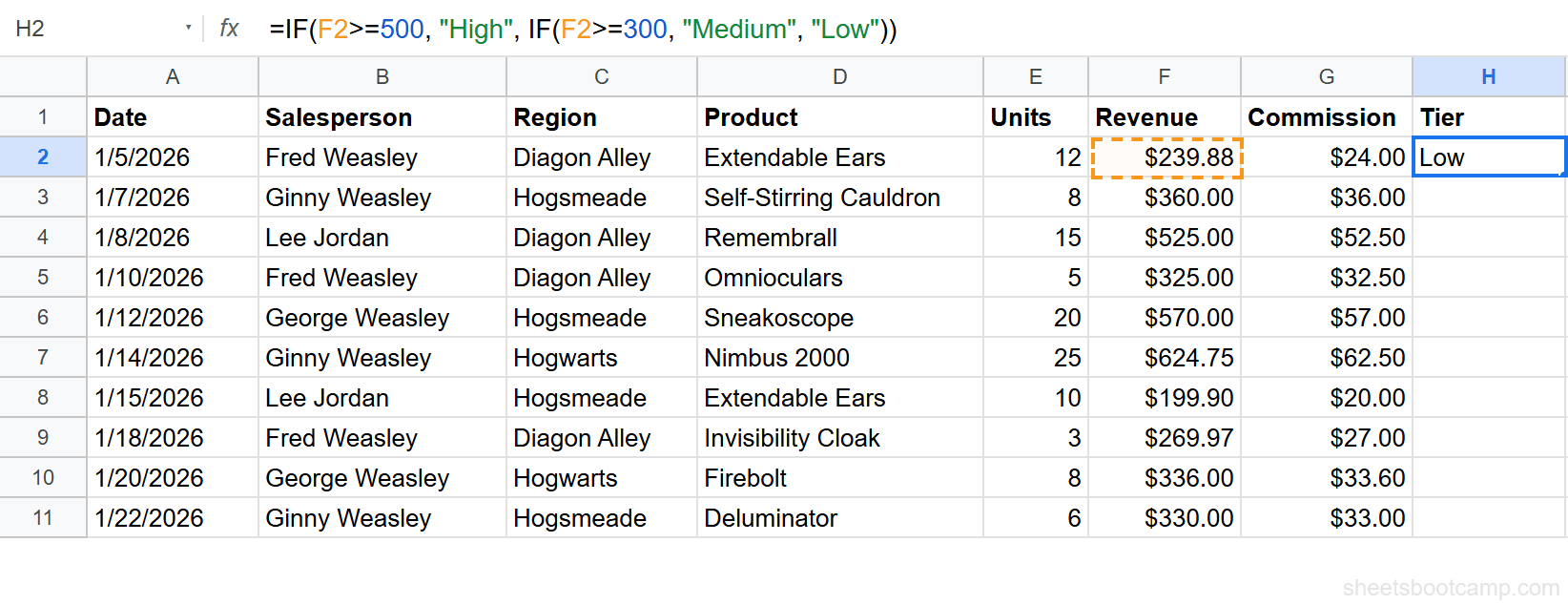
Select cell H2 and enter the following formula:
=IF(F2>=500, "High", IF(F2>=300, "Medium", "Low"))Press Enter. Cell H2 shows “Low” because F2 contains $239.88, which is less than 300.
Here is how Google Sheets evaluated this:
- Is $239.88 >= 500? No. Move to the inner IF.
- Is $239.88 >= 300? No. Return “Low.”
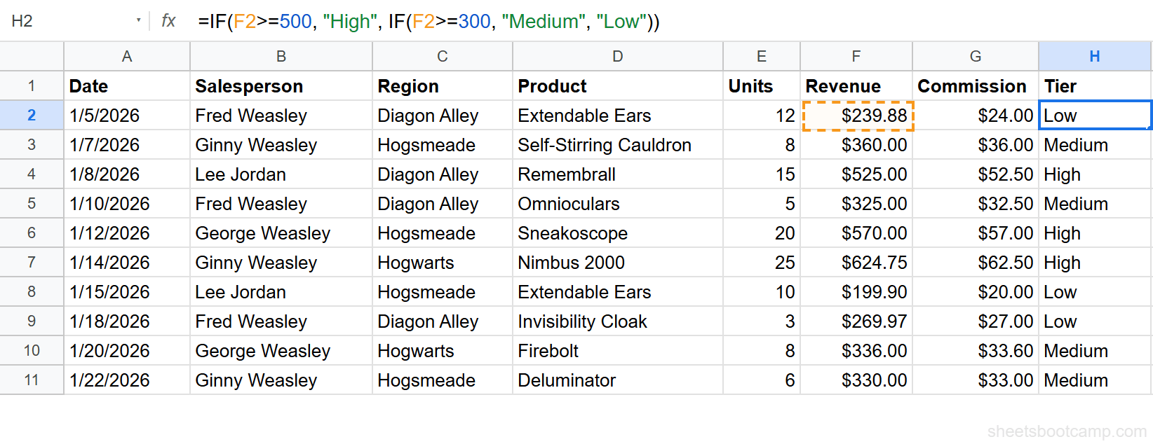
Copy the formula to all rows
Select H2 and drag the fill handle down through H11. Each row evaluates its own revenue value.
The results across all 10 rows:
| Salesperson | Revenue | Tier |
|---|---|---|
| Fred Weasley | $239.88 | Low |
| Ginny Weasley | $360.00 | Medium |
| Lee Jordan | $525.00 | High |
| Fred Weasley | $325.00 | Medium |
| George Weasley | $570.00 | High |
| Ginny Weasley | $624.75 | High |
| Lee Jordan | $199.90 | Low |
| Fred Weasley | $269.97 | Low |
| George Weasley | $336.00 | Medium |
| Ginny Weasley | $330.00 | Medium |
The fill handle is the small blue circle at the bottom-right corner of the selected cell. You can also copy H2, select H3:H11, and paste.
Example: 4-Tier Letter Grades
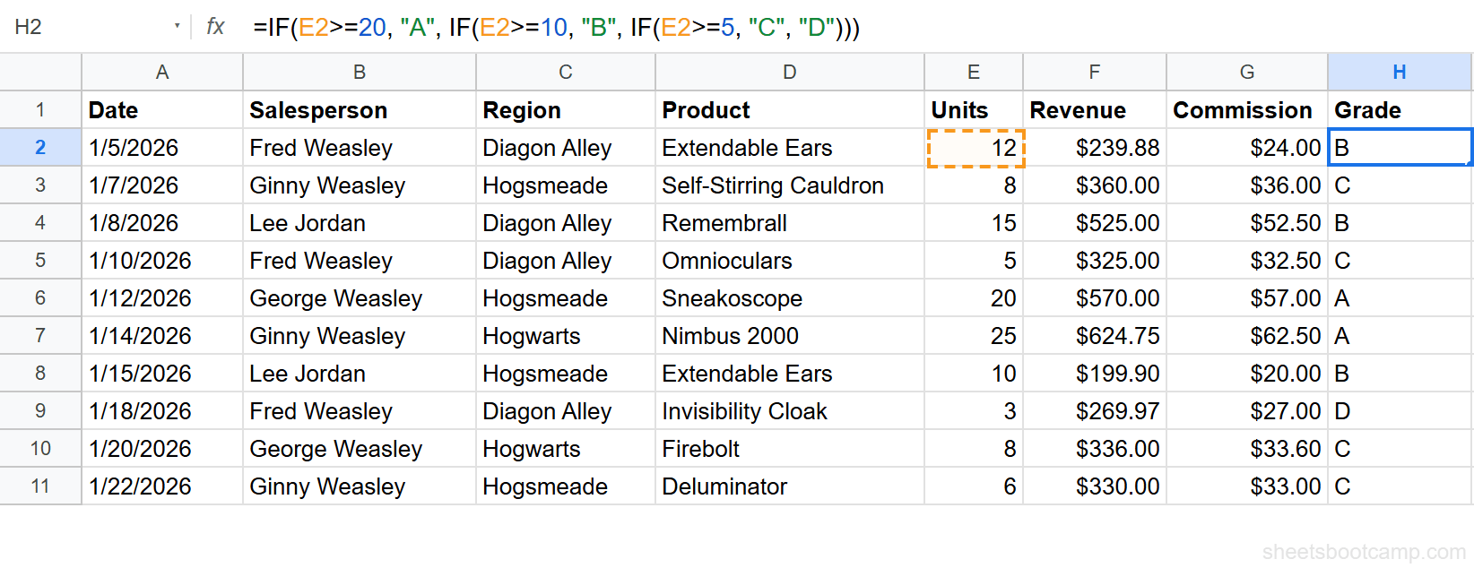
This example assigns a letter grade based on units sold (column E): A for 20+, B for 10-19, C for 5-9, and D for under 5.
=IF(E2>=20, "A", IF(E2>=10, "B", IF(E2>=5, "C", "D")))This formula nests three levels deep. Google Sheets checks each threshold in descending order:
- Is E2 >= 20? If yes, return “A.”
- Is E2 >= 10? If yes, return “B.”
- Is E2 >= 5? If yes, return “C.”
- None of the above? Return “D.”
For George Weasley’s 20 Sneakoscopes, this returns “A”. For Fred Weasley’s 3 Invisibility Cloaks, it returns “D”. Each closing parenthesis matches one of the three IF functions.
Example: Tiered Commission Rates
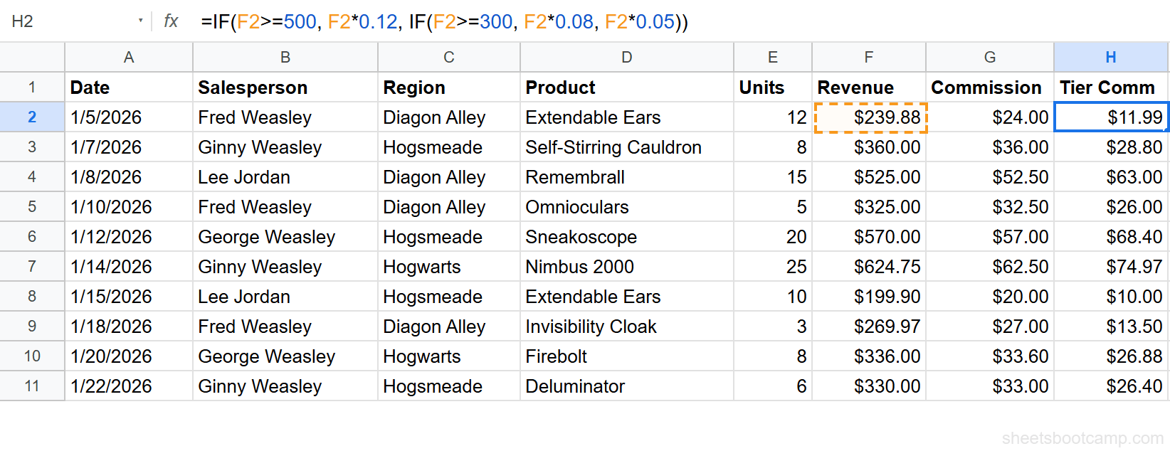
Instead of returning text labels, nested IF can return calculated values. This formula applies different commission percentages based on revenue: 12% for $500+, 8% for $300-$499, and 5% for under $300.
=IF(F2>=500, F2*0.12, IF(F2>=300, F2*0.08, F2*0.05))For Lee Jordan’s $525.00 sale, Google Sheets checks: is $525.00 >= 500? Yes. It returns $525.00 * 0.12 = $63.00. For Ginny Weasley’s $360.00 sale, the first condition is FALSE, so it checks the second: is $360.00 >= 300? Yes. It returns $360.00 * 0.08 = $28.80.
Format column H as currency after entering the formula. Select the column, then go to Format > Number > Currency.
Common Mistakes
Wrong Condition Order
The most frequent nested IF error is checking conditions in the wrong sequence. If you test >=300 before >=500, every value above 300 matches the first condition immediately. Values of 500, 600, or 1,000 all return “Medium” because Google Sheets never reaches the >=500 check.
Wrong:
=IF(F2>=300, "Medium", IF(F2>=500, "High", "Low"))This returns “Medium” for Lee Jordan’s $525.00 sale. The >=500 check is unreachable.
Correct:
=IF(F2>=500, "High", IF(F2>=300, "Medium", "Low"))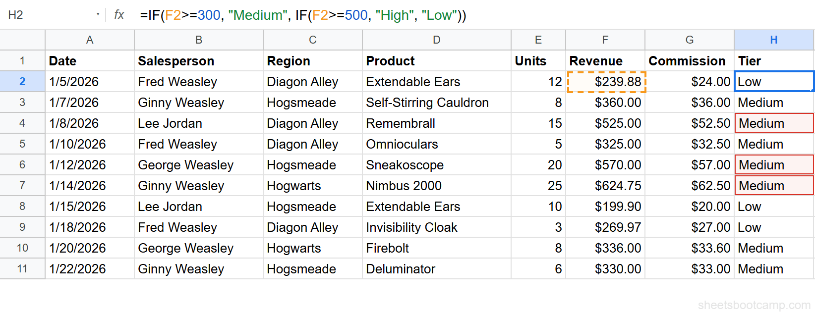
Google Sheets does not warn you about unreachable conditions. The formula runs without errors but produces wrong results. Always check your output against known values after writing a nested IF.
Missing Closing Parentheses
Each IF function needs its own closing parenthesis. Two nested IFs need two closing parentheses at the end. Three need three. If you miss one, Google Sheets shows a “Formula parse error” message.
Count the opening parentheses in your formula. The number of ) at the end should match the number of IF( statements.
Forgetting the Final Else Value
The last argument of the innermost IF is your catch-all default. If you omit it, Google Sheets returns FALSE as a literal value in the cell.
=IF(F2>=500, "High", IF(F2>=300, "Medium"))Any revenue under $300 displays the boolean FALSE instead of “Low.” Always include the final else value, even if it is an empty string "".
When to Stop Nesting
Three levels of nesting is a practical ceiling. At four or more levels, the formula becomes hard to read, hard to debug, and easy to break.
For 4+ conditions where each checks a different threshold, the IFS function is a cleaner choice. IFS takes pairs of conditions and results in a flat list:
=IFS(E2>=20, "A", E2>=10, "B", E2>=5, "C", TRUE, "D")Same logic, no nesting. The final TRUE, "D" acts as the default else.
For matching a single value against a list of exact matches (like mapping region codes to names), SWITCH is even more direct.
A quick rule: if your formula has more than 3 closing parentheses at the end, consider rewriting it with IFS.
Tips for Readable Nested IFs
-
Use line breaks in the formula bar. Press Ctrl+Enter (Cmd+Enter on Mac) inside the formula bar to add a new line. Breaking each IF onto its own line makes the structure visible.
-
Add cell notes as documentation. Right-click the cell with the formula and select “Insert note.” Describe what each tier represents. Future collaborators will thank you.
-
Consider helper columns for complex logic. If a nested IF depends on multiple conditions per tier, break those conditions into separate columns first. Then write a nested IF that references the helper column results instead of cramming everything into one formula.
-
Match your parentheses as you type. Google Sheets highlights matching parentheses when your cursor is next to one. Use this to verify each IF is properly closed before pressing Enter.
Related Google Sheets Tutorials
- IF Function in Google Sheets — Covers the basic IF syntax, step-by-step examples, and IF with AND and OR
- IFS Function in Google Sheets — Check multiple conditions without nesting, the recommended replacement for 4+ tiers
- IF with AND / OR in Google Sheets — Test multiple conditions at once using AND or OR inside a single IF
- VLOOKUP in Google Sheets — Look up values in a table when your data mapping is stored in a range instead of coded into a formula
FAQ
How many IF statements can you nest in Google Sheets?
Google Sheets does not publish a hard limit, but formulas can contain up to 30 nested IF functions. In practice, anything beyond 3 levels becomes difficult to read and debug. Use IFS for 4 or more conditions.
How does a nested IF formula work?
Google Sheets evaluates each condition from left to right. When it finds the first condition that is TRUE, it returns that result and stops. If no condition is TRUE, it returns the final else value. The order of your conditions determines which result wins.
What is the alternative to nested IF in Google Sheets?
The IFS function checks multiple conditions in a flat list without nesting. SWITCH matches a single value against a list of possible matches. Both are easier to read than deeply nested IF statements.
How do you use nested IF with text values?
Wrap text results in double quotes inside the formula. For example, =IF(A1>100, "High", IF(A1>50, "Medium", "Low")) returns the text strings High, Medium, or Low based on the value in A1.