
The default value has no case before it. It is a single argument at the end of the formula. If you accidentally add a case/value pair after the default, SWITCH treats your default as a case and the formula breaks silently.
beginner 7 min read
SWITCH Function in Google Sheets (With Examples)
Learn how to use the SWITCH function in Google Sheets to replace messy nested IFs. Includes full syntax breakdown, step-by-step examples, and error fixes.
SB
Sheets Bootcamp
March 1, 2026 · Updated May 22, 2026
Table of Contents
The SWITCH function in Google Sheets compares one value against a list of cases and returns the result for the first match. It replaces long chains of nested IF statements when you need to map specific values to specific outputs. We’ll cover the syntax, compare SWITCH to nested IF, walk through a real example with task status data, and show you how to avoid common errors.
In This Guide
- SWITCH Syntax and Parameters
- SWITCH vs Nested IF
- How to Map Status Labels with SWITCH: Step-by-Step
- SWITCH Examples
- Common Errors and How to Fix Them
- Tips and Best Practices
- Related Google Sheets Tutorials
- FAQ
SWITCH Syntax and Parameters
Here is the SWITCH formula structure in Google Sheets:
Formula
=SWITCH(expression, case1, value1, case2, value2, ..., [default]) SWITCH evaluates the expression once, then checks it against each case value in order. When it finds a match, it returns the corresponding value.
| Parameter | Description | Required |
|---|---|---|
| expression | The value to test. Can be a cell reference, formula, or literal value | Yes |
| case1 | The first value to compare against the expression | Yes |
| value1 | The result to return if expression matches case1 | Yes |
| case2, value2, … | Additional case/value pairs to check in sequence | No |
| default | The value returned if no case matches. Must be the last argument with no matching case before it | No |
Here is a real example. This formula checks the category in cell C2 and returns a department name:
Formula
=SWITCH(C2,"Optics","Sports","Laboratory","Alchemy","Surveillance","Sports","Accessories","General") If C2 contains “Laboratory”, this returns “Alchemy”. If C2 contains “Optics”, this returns “Sports”.
Important
SWITCH vs Nested IF
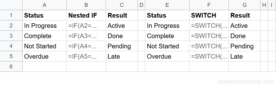
This is where SWITCH earns its place. Here is the same logic written both ways.
Mapping four status values with nested IF:
Formula
=IF(D2="Complete","Done",IF(D2="In Progress","Active",IF(D2="Not Started","Pending",IF(D2="Overdue","Late","Unknown")))) The same mapping with SWITCH:
Formula
=SWITCH(D2,"Complete","Done","In Progress","Active","Not Started","Pending","Overdue","Late","Unknown") Both return the same results. The SWITCH version is shorter, easier to scan, and does not require counting parentheses.
The difference grows with more cases. A nested IF with eight values requires seven levels of nesting and seven closing parentheses. SWITCH stays flat no matter how many cases you add.
When nested IF is the better choice: SWITCH only handles exact matches. If you need range-based conditions (greater than, less than, between), use nested IF or IFS instead. For example, classifying revenue as “High” when it exceeds $500 requires a comparison operator. SWITCH cannot do that.
| Feature | SWITCH | Nested IF |
|---|---|---|
| Exact value matching | Yes | Yes |
| Range-based conditions | No | Yes |
| Readability with 4+ cases | Clean, flat structure | Deeply nested, hard to read |
| Default / else value | Optional last argument | Built-in third argument |
| Expression evaluated | Once | Once per level |
How to Map Status Labels with SWITCH: Step-by-Step
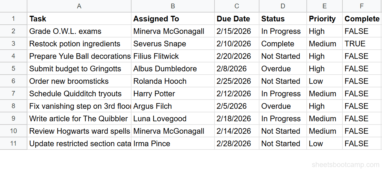
We’ll use a task tracker with 10 rows. The goal: map each task’s Status value (“In Progress”, “Complete”, “Not Started”, “Overdue”) to a shorter label using SWITCH.
1
Set up your data
Your spreadsheet has task data in columns A through F. Column D contains the Status values. You will add the SWITCH formula in column G.
2
Enter the SWITCH formula
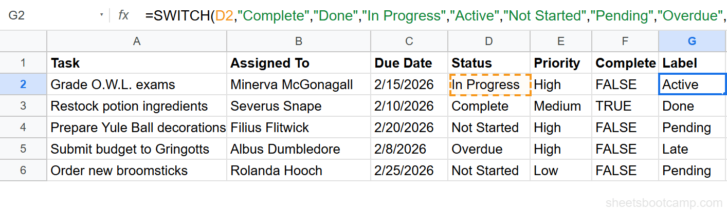
Select cell G2 and enter this formula:
Formula
=SWITCH(D2,"Complete","Done","In Progress","Active","Not Started","Pending","Overdue","Late","Unknown") This checks the value in D2 against four cases:
- “Complete” returns “Done”
- “In Progress” returns “Active”
- “Not Started” returns “Pending”
- “Overdue” returns “Late”
- If none match, the default returns “Unknown”
D2 contains “In Progress”, so the formula returns “Active”.
Tip
SWITCH matches text without case sensitivity. “in progress” and “In Progress” both match the same case. You do not need to worry about capitalization in your data.
3
Review the result and fill down
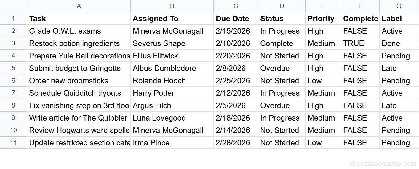
Drag the fill handle from G2 down to G11 to apply the formula to all 10 rows. Here are the results:
- “In Progress” returns “Active” (rows 1, 6, 8, 11)
- “Complete” returns “Done” (rows 2, 12)
- “Not Started” returns “Pending” (rows 3, 5, 9, 10)
- “Overdue” returns “Late” (rows 4, 7)
Every status value maps to the correct label. No row returns “Unknown” because all values match a defined case.
SWITCH Examples
Example 1: Category Discount Rates
You have a product inventory and want to assign discount rates by category. Column C contains the category name.
Formula
=SWITCH(C2,"Optics",0.15,"Laboratory",0.10,"Surveillance",0.20,"Espionage",0.05,0) For SKU-101 (Optics), this returns 0.15 (15% discount). For SKU-108 (Espionage), this returns 0.05. For SKU-103 (Accessories), no case matches, so the default returns 0 (no discount).
To calculate the discounted price, combine SWITCH with arithmetic:
Formula
=D2*(1-SWITCH(C2,"Optics",0.15,"Laboratory",0.10,"Surveillance",0.20,"Espionage",0.05,0)) For SKU-101 ($24.99 at 15% off), this returns $21.24. For SKU-104 ($65.00 at 20% off), this returns $52.00.
Example 2: Region Codes from Full Names
Your sales records have full region names in column C. You need three-letter codes for a report.
Formula
=SWITCH(C2,"North","NOR","South","SOU","East","EST","West","WST","OTH") Each region name maps to its code. The default “OTH” catches any region not in the list. This is cleaner than writing four nested IFs for a lookup that may grow over time.
Example 3: SWITCH with a Calculated Expression
SWITCH does not require a cell reference as the expression. You can pass a formula result.
Formula
=SWITCH(WEEKDAY(A2),1,"Weekend",7,"Weekend","Weekday") WEEKDAY returns 1 for Sunday and 7 for Saturday. This formula checks the day-of-week number and returns “Weekend” for those two values. Everything else hits the default and returns “Weekday”.
Common Errors and How to Fix Them
#N/A Error (No Match Found)
SWITCH returns #N/A when the expression does not match any case and no default value is provided.
Formula
=SWITCH(D2,"Complete","Done","In Progress","Active") If D2 contains “Overdue”, this formula returns #N/A because “Overdue” is not listed as a case and there is no default. Add a default value as the last argument:
Formula
=SWITCH(D2,"Complete","Done","In Progress","Active","Other") Now unmatched values return “Other” instead of #N/A.
#VALUE! Error (Wrong Number of Arguments)
SWITCH requires at least three arguments: the expression, one case, and one value. If you pass an even number of arguments after the expression without intending a default, Google Sheets may misinterpret the last case as a default.
Double-check that every case has a paired value. If you want a default, it should be a single unpaired argument at the end.
Unexpected Results from Extra Spaces
If your data contains trailing spaces (“Complete ” instead of “Complete”), SWITCH will not match the case. The values look identical on screen but the space makes them different strings.
Wrap the expression in TRIM to strip extra spaces:
Formula
=SWITCH(TRIM(D2),"Complete","Done","In Progress","Active","Not Started","Pending","Overdue","Late","Unknown") Tip
Wrap your SWITCH in IFERROR if you cannot guarantee all values have a matching case. Use =IFERROR(SWITCH(D2,"Complete","Done"),"Unknown") as a safety net, though adding a proper default inside SWITCH is the better approach.
Tips and Best Practices
-
Always include a default value. The default is the last unpaired argument in SWITCH. Without it, unmatched values return #N/A. Even if you expect all values to match, a default catches data entry mistakes.
-
Use SWITCH for exact matches only. SWITCH compares the expression to each case using exact equality. For conditions involving greater than, less than, or between, use IFS or nested IF instead.
-
Keep it under 10 cases. SWITCH works well for small value maps. If your mapping has 10 or more entries, move the lookup data to a reference range and use VLOOKUP or INDEX MATCH. A reference range is easier to maintain and update.
-
Combine SWITCH with other functions. You can nest SWITCH inside ARRAYFORMULA, use it inside FILTER criteria, or wrap the expression in functions like TRIM, UPPER, or WEEKDAY to transform the value before matching.
-
SWITCH evaluates the expression once. Unlike nested IF, which re-evaluates the cell reference at each level, SWITCH evaluates the expression a single time and compares the result against each case. For formulas with expensive calculations as the expression, SWITCH is more efficient.
Note
SWITCH is available in Google Sheets and Excel 2019+. If you share workbooks with users on older Excel versions, they will see a compatibility error. Use nested IF or IFS as a fallback.
Related Google Sheets Tutorials
- IF Statements in Google Sheets - Learn the foundational IF function and when to use it
- Nested IF Statements - Handle multiple conditions with nested IF when you need range-based logic
- IFS Function - Evaluate multiple conditions in a flat list without nesting
- IF with AND, OR, NOT - Combine logical operators for multi-condition tests
- VLOOKUP in Google Sheets - Look up values from a reference range when your mapping table is large
Frequently Asked Questions
What does the SWITCH function do in Google Sheets?
SWITCH compares one expression against a list of values and returns the result for the first match. It works like a lookup table inside a formula, checking the expression against each case value in order.
What is the difference between SWITCH and nested IF?
Nested IF tests a series of logical conditions (greater than, less than, equals). SWITCH compares a single expression against exact values. Use SWITCH when you are matching specific values like status codes or category names. Use nested IF when you need range-based conditions.
Does SWITCH work with numbers and text?
Yes. SWITCH matches both text strings and numbers. For text comparisons, SWITCH is not case-sensitive. It treats "Complete" and "complete" as the same value.
What happens if no case matches in SWITCH?
If you included a default value, SWITCH returns that. If you did not include a default, SWITCH returns #N/A. Always add a default value as the last argument to prevent unexpected errors.
Can I use SWITCH instead of VLOOKUP?
For small lookup tables with fewer than 10 values, SWITCH works well and keeps everything inside one formula. For larger reference tables or data that changes often, VLOOKUP or INDEX MATCH is a better choice because the lookup range updates automatically.
You've googled this formula before. Probably more than once.
The Bootcamp is a real Google Sheet that grades every formula the moment you press Enter. 193 exercises across 9 modules, the 10% of Sheets that does 90% of the work. One payment of $29.
Get It for $29 Get the Bootcamp for $2930-day refund. Reply to any email and you get your money back.
Not ready to pay? Try Basic Training free →