How to Insert an Image in a Cell in Google Sheets
Learn how to insert an image inside a cell in Google Sheets using the IMAGE function and the Insert menu. Covers sizing modes, URLs, and troubleshooting.
Sheets Bootcamp
March 1, 2026 · Updated June 25, 2026
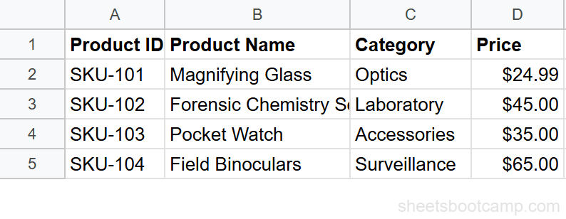
The IMAGE function in Google Sheets inserts an image inside a cell from a URL. The image lives in the cell, moves when you sort or filter, and scales when you resize the row or column. It’s the formula-based way to add product photos, flags, icons, or charts directly into your data.
This guide covers the IMAGE function syntax, all four sizing modes, the Insert menu alternative, and how to fix common URL issues.
In This Guide
- What Is the IMAGE Function?
- Syntax and Parameters
- How to Insert an Image: Step-by-Step
- IMAGE Examples
- Common Errors and How to Fix Them
- Tips and Best Practices
- Related Google Sheets Tutorials
- FAQ
What Is the IMAGE Function?
IMAGE takes a URL that points to an image file and displays that image inside the cell. Unlike inserting an image over cells (which floats on top of the grid), an in-cell image is part of the data. It sorts, filters, and copies with the row.
This is useful for product catalogs, employee directories, country flag tables, or any dataset where a visual identifier makes the data easier to scan.
Syntax and Parameters
=IMAGE(url, [mode], [height], [width])| Parameter | Description | Required |
|---|---|---|
| url | The URL of the image (must be publicly accessible and in quotes) | Yes |
| mode | Sizing mode: 1 (fit, default), 2 (stretch), 3 (original), 4 (custom) | No |
| height | Height in pixels (only used with mode 4) | No |
| width | Width in pixels (only used with mode 4) | No |
Sizing Modes
| Mode | Behavior |
|---|---|
| 1 (default) | Scales the image to fit inside the cell while maintaining aspect ratio. Extra space is left blank |
| 2 | Stretches the image to fill the cell completely. May distort the aspect ratio |
| 3 | Displays the image at its original size. May be cropped if the cell is smaller |
| 4 | Custom size. You specify height and width in pixels |
The URL must point directly to an image file — not to a web page containing an image. URLs from Google Drive need to be converted to the direct download format. A Google Drive share link alone won’t work.
How to Insert an Image: Step-by-Step
We’ll add a product image to a cell using the IMAGE function.
Get the image URL
Find the direct URL of the image. For web images, right-click the image and select Copy image address. The URL should point directly to the image file (ending in .png, .jpg, or similar).
Enter the IMAGE formula
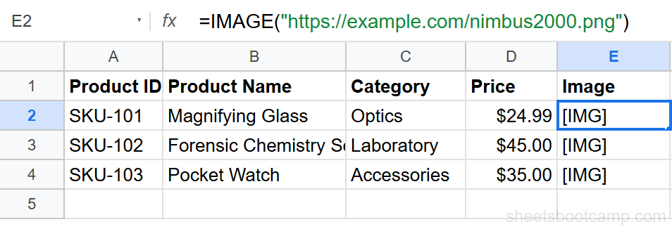
Click the cell where you want the image (e.g., E2). Enter the formula with the URL in quotes:
=IMAGE("https://upload.wikimedia.org/wikipedia/en/thumb/7/7d/Example_image.png/220px-Example_image.png")Press Enter. The image appears inside the cell, scaled to fit.
Adjust the cell size
Drag the row height border to make the cell taller. The image scales proportionally with the cell. For a consistent look across rows, select all data rows and set a fixed row height via Format > Row height.
You can also insert an image without a formula: go to Insert > Image > Image in cell. This opens a dialog where you can upload from your computer, paste a URL, or search the web. The result is the same — the image lives inside the cell.
IMAGE Examples
Display Images from a URL Column
Store image URLs in column E and display them in column F using the formula:
=IMAGE(E2)No quotes needed because E2 already contains the URL text. Copy the formula down the column to display images for every row.
Use a Specific Size (Mode 4)
Display an image at exactly 50 pixels high and 50 pixels wide:
=IMAGE("https://example.com/icon.png", 4, 50, 50)Mode 4 ignores the cell size and renders the image at the specified dimensions. This is useful for creating uniform icon columns.
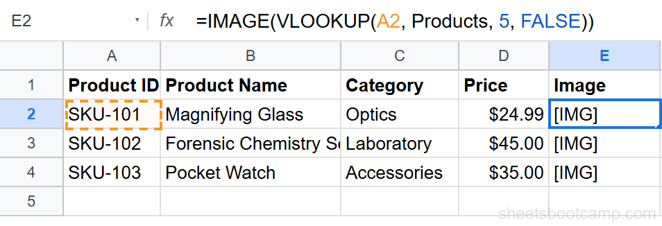
Combine IMAGE with VLOOKUP
Look up a product name and display its image. If column E in your Products table contains image URLs:
=IMAGE(VLOOKUP(A2, Products, 5, FALSE))This retrieves the URL from the Products table using VLOOKUP and passes it to IMAGE. When A2 changes, the displayed image updates automatically.
Use Google Drive Images
For images stored in Google Drive, convert the share link to a direct URL format:
=IMAGE("https://drive.google.com/uc?id=FILE_ID")Replace FILE_ID with the actual file ID from the share URL. The file must have “Anyone with the link” sharing permissions.
Common Errors and How to Fix Them
Empty Cell (No Error, No Image)
The URL is valid but doesn’t point to a publicly accessible image. Check that the image isn’t behind a login wall, firewall, or requires authentication. Google Drive files must be shared with “Anyone with the link.”
#VALUE! Error
The URL argument is missing or the mode/height/width arguments are invalid. Verify the URL is enclosed in quotes (if typed directly) and that mode is 1, 2, 3, or 4.
Image Appears Distorted
You’re using mode 2 (stretch), which ignores aspect ratio. Switch to mode 1 (default) to maintain proportions, or use mode 4 with specific height and width values that match the image’s aspect ratio.
Test image URLs by pasting them directly into your browser’s address bar. If the image loads in the browser, it will work in the IMAGE function. If the browser shows a web page instead of an image, the URL isn’t a direct image link.
Tips and Best Practices
-
Use mode 1 for most cases. The default fit-to-cell mode maintains aspect ratio and looks clean. Mode 2 distorts images, and mode 3 may crop them.
-
Set consistent row heights for image columns. Select all rows with images and set the same height (e.g., 80px) via Format > Row height. This gives your data a catalog-like appearance.
-
Store URLs in a separate column. Keep image URLs in one column and the IMAGE formula in the next. This separates data from display and makes it easier to update URLs without editing formulas.
-
Use HTTPS URLs. Google Sheets requires HTTPS for image URLs. HTTP links may fail silently, showing an empty cell instead of an error.
-
Watch for rate limits on external images. If you’re loading many images from the same server, some may fail to display. The server may block rapid requests. Use a CDN or host images on Google Drive for reliable loading.
Related Google Sheets Tutorials
- VLOOKUP: The Complete Guide - Look up image URLs dynamically and pass them to the IMAGE function
- Data Validation: The Complete Guide - Create dropdown selections that trigger IMAGE formulas for product catalogs
- Conditional Formatting: The Complete Guide - Highlight cells around images based on data values
- ARRAYFORMULA Complete Guide - Apply the IMAGE function across an entire column with a single formula
FAQ
How do I put an image inside a cell in Google Sheets?
Use the IMAGE function: =IMAGE("url"). The image fits inside the cell and moves with it. You can also go to Insert > Image > Image in cell, which opens a dialog to upload, search, or paste a URL.
What is the difference between image in cell and image over cells?
An image in cell lives inside a single cell — it moves and resizes with the cell. An image over cells floats above the grid like a text box — it can span multiple cells and doesn’t shift when rows or columns are resized.
Why does the IMAGE function show an error?
The URL is invalid, inaccessible, or not a direct image link. Some URLs point to web pages that contain images rather than the image file itself. Make sure the URL links directly to the image file. Also check that the image is publicly accessible — private or login-protected images won’t load.
Can I use the IMAGE function with VLOOKUP?
Yes. Store image URLs in a column, then use VLOOKUP to retrieve the URL and wrap it in IMAGE: =IMAGE(VLOOKUP(A2, Products, 5, FALSE)). This dynamically displays the product image matching the lookup value.
What image formats does Google Sheets support?
The IMAGE function supports PNG, JPG, GIF (including animated), BMP, ICO, and SVG formats. The image must be hosted at a publicly accessible URL. Data URIs and local file paths don’t work.
How do I resize an image in a cell?
Change the row height and column width — the image scales with the cell in the default mode. For exact control, use mode 4: =IMAGE("url", 4, height, width) where height and width are in pixels.