INDEX MATCH Closest Value in Google Sheets
Find the closest value in Google Sheets using INDEX MATCH. Covers nearest match with MIN ABS, next lower, next higher, and closest date formulas with examples.
Sheets Bootcamp
March 4, 2026 · Updated October 5, 2026
INDEX MATCH in Google Sheets handles exact lookups well, but sometimes you need the closest value rather than a perfect match. Finding the nearest number, the closest date, or the next price tier below a budget all require approximate matching techniques that go beyond match_type: 0. This guide covers three approaches: the absolute closest value using MIN and ABS, the next lower value, and the next higher value, with step-by-step examples using monthly sales data.
In This Guide
- Why Closest Value Matching Matters
- Closest Value with MIN and ABS: Step-by-Step
- Next Lower Value (Floor Match)
- Next Higher Value (Ceiling Match)
- Closest Date Match
- Example: Closest Price to a Budget
- XLOOKUP Alternative
- Common Errors and Fixes
- Tips
- Related Google Sheets Tutorials
- Frequently Asked Questions
Why Closest Value Matching Matters
Exact matches work when your search key exists in the data. When it does not, MATCH with match_type: 0 returns #N/A. That is fine if an exact match is required, but many real scenarios need the nearest value instead:
- Finding which month hit closest to a revenue target
- Matching a budget to the nearest available price
- Looking up the closest date to a deadline
- Assigning values to the nearest bracket or tier
Google Sheets gives you three options depending on what “closest” means for your situation.
Closest Value with MIN and ABS: Step-by-Step
This approach finds the value with the smallest absolute difference from your target, regardless of whether it is above or below. The data does not need to be sorted.
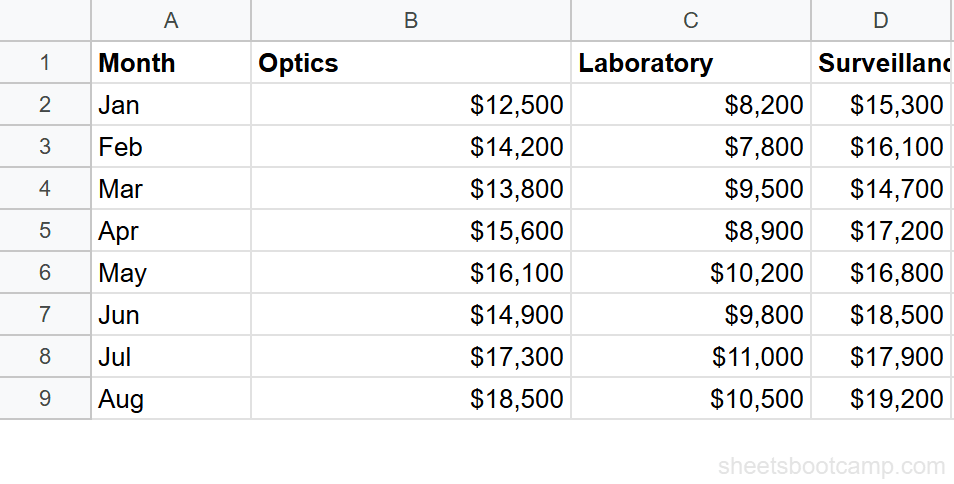
Sample Data
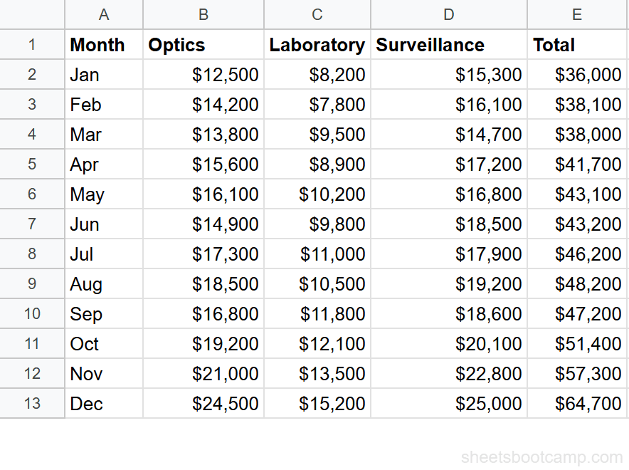
The monthly summary has 12 rows of sales data. Column A contains the month, columns B through D hold category sales (Optics, Laboratory, Surveillance), and column E has the Total. Totals range from $36,000 in January to $64,700 in December.
The Formula
=INDEX(A2:A13, MATCH(MIN(ABS(E2:E13-H2)), ABS(E2:E13-H2), 0))Here is what each part does:
ABS(E2:E13-H2)calculates the absolute difference between every Total value and the target in H2. This produces an array of 12 distances.MIN(...)finds the smallest distance in that array.MATCH(..., 0)locates the position of that smallest distance.INDEX(A2:A13, ...)returns the month at that position.
This formula uses array operations. Either wrap it with ARRAYFORMULA as =INDEX(A2:A13, MATCH(ARRAYFORMULA(MIN(ABS(E2:E13-H2))), ARRAYFORMULA(ABS(E2:E13-H2)), 0)) or press Ctrl+Shift+Enter after typing the formula. Without one of these approaches, the ABS function processes only the first cell instead of the full range.
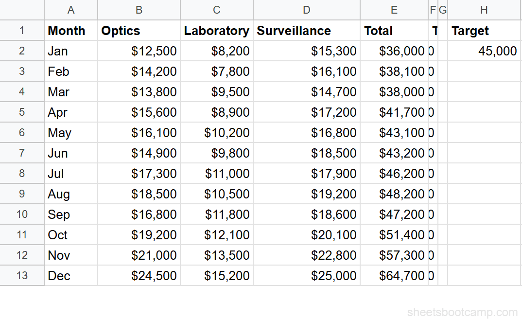
Set up your data and target value
The monthly summary runs from A1:E13. Enter a target value of 45000 in cell H2.
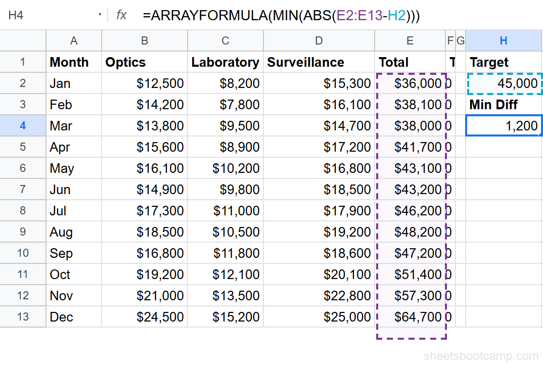
Write the MIN ABS formula to find the smallest difference
In cell H4, enter:
=ARRAYFORMULA(MIN(ABS(E2:E13-H2)))This returns 1,200, the smallest absolute difference between any Total and 45,000. July’s total of $46,200 is $1,200 away from the target, and no other month is closer.
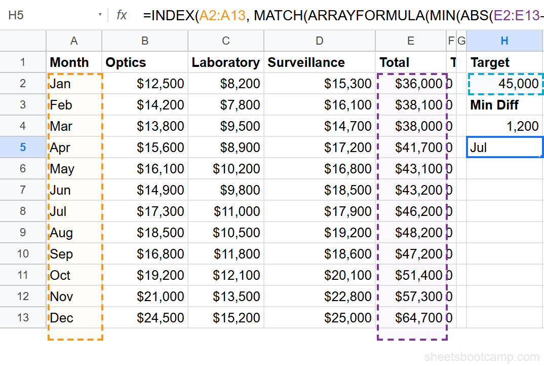
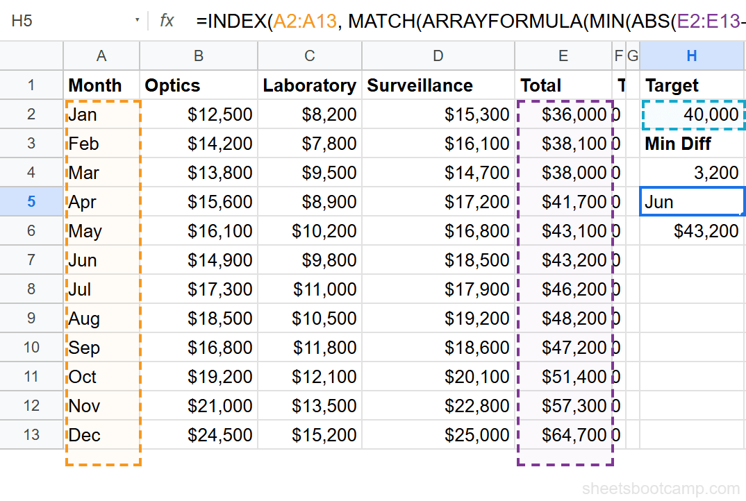
Combine INDEX MATCH with MIN ABS
In cell H5, enter the full formula:
=INDEX(A2:A13, MATCH(ARRAYFORMULA(MIN(ABS(E2:E13-H2))), ARRAYFORMULA(ABS(E2:E13-H2)), 0))This returns Jul. The MATCH function found the position of the 1,200 difference in the ABS array (position 7), and INDEX pulled “Jul” from the Month column at that position.
Return the matching value alongside the label
In cell H6, get the actual closest total:
=INDEX(E2:E13, MATCH(ARRAYFORMULA(MIN(ABS(E2:E13-H2))), ARRAYFORMULA(ABS(E2:E13-H2)), 0))This returns $46,200, confirming that July is the closest month. The target was $45,000, and $46,200 is $1,200 above it.
Test with a different target
Change H2 to 40000. The month formula updates to Jun ($43,200 total, difference of $3,200). Change it to 50000 and the result becomes Oct ($51,400 total, difference of $1,400). The formula recalculates automatically.
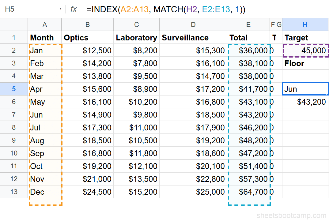
Next Lower Value (Floor Match)
When you need the nearest value that is less than or equal to your target, use match_type: 1 in MATCH. This is useful for tax brackets, pricing tiers, and shipping thresholds where you want the floor.
=INDEX(A2:A13, MATCH(H2, E2:E13, 1))MATCH with match_type: 1 finds the largest value in E2:E13 that is less than or equal to H2.
Match type 1 requires column E to be sorted in ascending order. If the data is not sorted, the formula returns wrong results without any error message. Sort the lookup column before using this approach.
With the monthly summary data, the Total column already increases from January ($36,000) to December ($64,700), so the data is in ascending order. If H2 is 45000, MATCH returns position 6, because $43,200 (June) is the largest total that does not exceed $45,000. INDEX then returns Jun.
Next Higher Value (Ceiling Match)
For the nearest value greater than or equal to your target, use match_type: -1. This applies to minimum order quantities, deadline lookups, and next-available-slot scenarios.
=INDEX(A2:A13, MATCH(H2, E2:E13, -1))Match type -1 requires the data sorted in descending order. The monthly summary is sorted ascending, so you would need to sort it descending (or reference a separate descending-sorted range) before using this approach.
If you sort the Total column from highest to lowest, the formula with match_type: -1 and a target of 45000 returns the first value that is greater than or equal to 45000. That would be Jul ($46,200).
For most situations, the MIN ABS approach from the previous section is more practical because it works on unsorted data and finds the true closest value regardless of direction.
Closest Date Match
Dates in Google Sheets are stored as serial numbers (January 1, 1900 = 1), so the MIN ABS pattern works on dates the same way it works on revenue figures. The VLOOKUP with dates logic is identical: subtract the target date from each date in the range, take the absolute value, and find the minimum.
Suppose column A contains dates and column B contains event names. To find the event closest to a target date in D2:
=INDEX(B2:B20, MATCH(ARRAYFORMULA(MIN(ABS(A2:A20-D2))), ARRAYFORMULA(ABS(A2:A20-D2)), 0))The formula works because the date subtraction produces a number of days, and MIN finds the smallest gap. A gap of 0 means an exact date match. A gap of 3 means the closest event is 3 days away.
If two values are equally close to the target (one above, one below), MATCH returns the first one it encounters in the range. To control tie-breaking, sort your data so the preferred direction appears first.
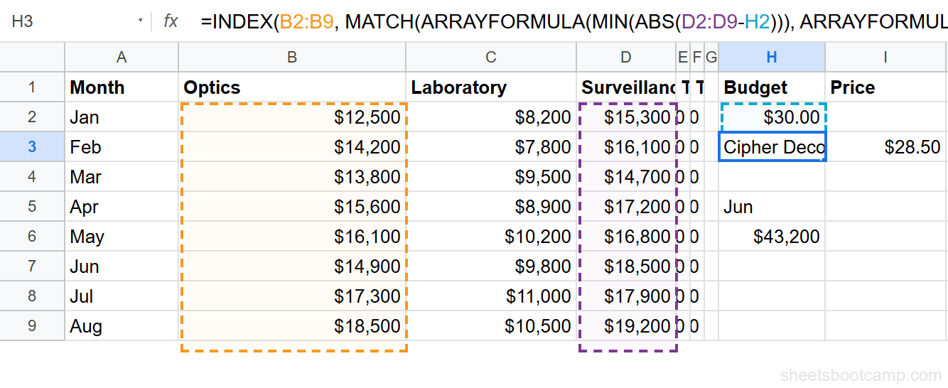
Example: Closest Price to a Budget
Using the product inventory data, find the product with the price closest to a budget of $30.00. The inventory has 12 products with prices ranging from $12.50 (Calligraphy Pen) to $89.99 (Disguise Kit).
The budget is $30.00, entered in cell H2. Enter this formula:
=INDEX(B2:B13, MATCH(ARRAYFORMULA(MIN(ABS(D2:D13-H2))), ARRAYFORMULA(ABS(D2:D13-H2)), 0))This returns Cipher Decoder. The Cipher Decoder costs $28.50, which is $1.50 away from the $30.00 budget. The next closest is the Pocket Watch at $35.00 ($5.00 away).
To confirm, pull the price in a neighboring cell:
=INDEX(D2:D13, MATCH(ARRAYFORMULA(MIN(ABS(D2:D13-H2))), ARRAYFORMULA(ABS(D2:D13-H2)), 0))This returns $28.50.
XLOOKUP Alternative
Google Sheets added XLOOKUP, which includes a match_mode argument for approximate matching. XLOOKUP can find the next smaller value (match_mode: -1) or the next larger value (match_mode: 1) without requiring sorted data.
=XLOOKUP(H2, E2:E13, A2:A13, "Not found", -1)This returns the month whose Total is the next value below the target. XLOOKUP handles the floor and ceiling cases more cleanly than MATCH with match_type: 1 or -1, because XLOOKUP does not require the data to be sorted.
However, XLOOKUP does not have a built-in “absolute closest” mode. For finding the true nearest value regardless of direction, the INDEX MATCH MIN ABS pattern remains the go-to approach.
Common Errors and Fixes
#VALUE! Error
The ABS(range - target) operation breaks if any cell in the range contains text instead of a number. Check that the lookup column has no text values, blank headers, or mixed data types. Filter your range to include only the numeric data rows.
#N/A Error
MATCH returns #N/A when no match is found. With the MIN ABS pattern, this usually means the ABS array did not evaluate correctly. Confirm that you used ARRAYFORMULA or pressed Ctrl+Shift+Enter. Without array processing, ABS only evaluates the first cell and MIN returns a single difference that might not appear in the full ABS array.
Wrong Result from Match Type 1 or -1
If the floor or ceiling formula returns an unexpected value, the data is not sorted in the required order. Match type 1 needs ascending order. Match type -1 needs descending order. Sort the lookup column first, or switch to the MIN ABS approach which works on unsorted data.
Tips
-
Use named ranges for clarity.
=INDEX(Months, MATCH(ARRAYFORMULA(MIN(ABS(Totals-Target))), ARRAYFORMULA(ABS(Totals-Target)), 0))is easier to read than cell references, especially when the formula appears in multiple places. -
Return multiple columns. Change the INDEX range to pull any column from the matched row. Use
INDEX(B2:B13, ...)for one column, orINDEX(A2:E13, ..., column_number)for a specific column from a wider range. -
Handle ties deliberately. When two values are equally close, MATCH returns the first match in the range. If you prefer the lower or higher value, sort your data accordingly before applying the formula.
-
Prefer MIN ABS over match_type 1 and -1 when you want the true closest value. The floor and ceiling approaches are useful for bracket lookups, but MIN ABS is the general-purpose solution.
Related Google Sheets Tutorials
- INDEX MATCH in Google Sheets - Full guide to the INDEX MATCH pattern, including syntax, examples, and when to use it over VLOOKUP
- INDEX MATCH for Beginners - Step-by-step introduction to how MATCH and INDEX work individually and together
- INDEX MATCH with Multiple Criteria - Look up values based on two or more conditions using array multiplication
- VLOOKUP with Dates - Use VLOOKUP to search for dates, including approximate date matching with sorted data
Frequently Asked Questions
How do I find the closest value in Google Sheets?
Use INDEX MATCH with MIN and ABS. The formula =INDEX(return_range, MATCH(MIN(ABS(data_range-target)), ABS(data_range-target), 0)) finds the value in the data range that is closest to the target number. Wrap the ABS arrays in ARRAYFORMULA or press Ctrl+Shift+Enter.
Does INDEX MATCH support approximate matching?
Yes. Set the match_type argument in MATCH to 1 for the next lower value or -1 for the next higher value. Match type 1 requires data sorted in ascending order, and -1 requires descending order.
Can I find the closest date with INDEX MATCH?
Yes. Dates in Google Sheets are numbers, so the MIN ABS formula works on dates the same way it works on numbers. Use =INDEX(return_range, MATCH(MIN(ABS(date_range-target_date)), ABS(date_range-target_date), 0)) with ARRAYFORMULA.
What is the difference between match_type 1 and match_type 0 in MATCH?
Match type 0 finds an exact match only. Match type 1 finds the largest value less than or equal to the search key, and the data must be sorted ascending. Match type -1 finds the smallest value greater than or equal to the search key, requiring descending order.
Can XLOOKUP find the closest value in Google Sheets?
XLOOKUP supports approximate matching with its match_mode argument. Set match_mode to 1 for the next larger value or -1 for the next smaller value. For the absolute closest value, the INDEX MATCH MIN ABS pattern is still needed.