INDEX MATCH Multiple Criteria in Google Sheets
Use INDEX MATCH with multiple criteria in Google Sheets to look up values based on two or more conditions. Array formula examples with step-by-step setup.
Sheets Bootcamp
March 14, 2026
Standard INDEX MATCH searches one column for one value. When you need to match on two or more conditions — like a specific Product ID in a specific Category — you multiply condition arrays inside MATCH and search for 1. This guide covers the array formula pattern, walks through building a multi-criteria lookup step by step, and shows practical examples with the product inventory data.
In This Guide
- How Multi-Criteria INDEX MATCH Works
- Two-Criteria Lookup: Step-by-Step
- Practical Examples
- Three or More Criteria
- Compared to VLOOKUP with a Helper Column
- Common Errors
- Tips
- Related Google Sheets Tutorials
- Frequently Asked Questions
How Multi-Criteria INDEX MATCH Works
The standard INDEX MATCH formula searches for one value:
=INDEX(return_range, MATCH(search_key, lookup_range, 0))For multiple criteria, replace the single search with an array multiplication pattern:
=INDEX(return_range, MATCH(1, (criteria1)*(criteria2), 0))Here is what happens inside the formula:
-
Each condition creates an array of TRUE/FALSE values.
(A2:A9="SKU-107")produces{FALSE, FALSE, FALSE, FALSE, FALSE, FALSE, TRUE, FALSE}— TRUE only where the Product ID matches. -
Multiplying arrays converts TRUE to 1 and FALSE to 0. When you multiply two arrays, the result is 1 only where both conditions are TRUE. Everywhere else, the result is 0.
-
MATCH searches for 1. The first
1in the multiplied array marks the row where all conditions matched. -
INDEX returns the value at that position from the return range.
The formula searches for 1 rather than the actual value because 1 represents the intersection of all TRUE conditions.
In current versions of Google Sheets, this formula works with a regular Enter press. Older versions may require Ctrl+Shift+Enter to enter it as an array formula. If the formula returns an error, try Ctrl+Shift+Enter.
Two-Criteria Lookup: Step-by-Step
We’ll find the price for a product that matches both a Product ID and a Category in the product inventory.
Sample Data
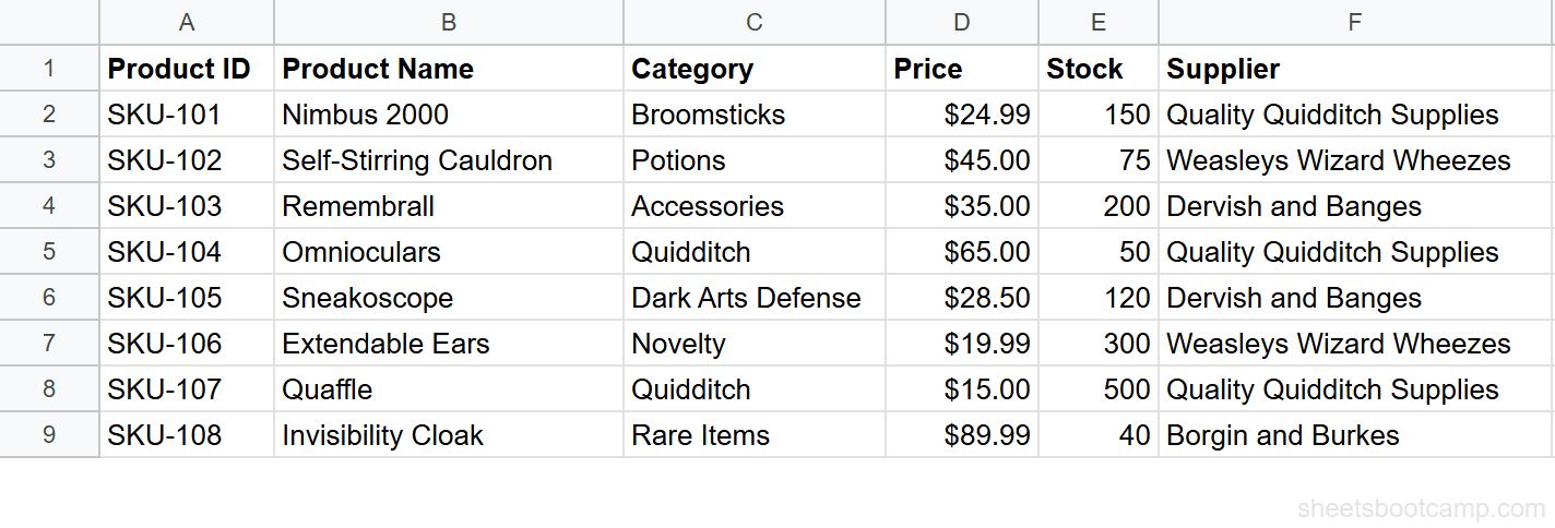
The inventory has 8 products with Product ID (A), Product Name (B), Category (C), Price (D), Stock (E), and Supplier (F).
Set up your data
The product inventory runs from A1:F9, with headers in row 1 and data in rows 2 through 9. We want to find the price for Product ID SKU-107 in the Quidditch category.
Identify the criteria
Two conditions must both be true:
- Column A (Product ID) = “SKU-107”
- Column C (Category) = “Quidditch”
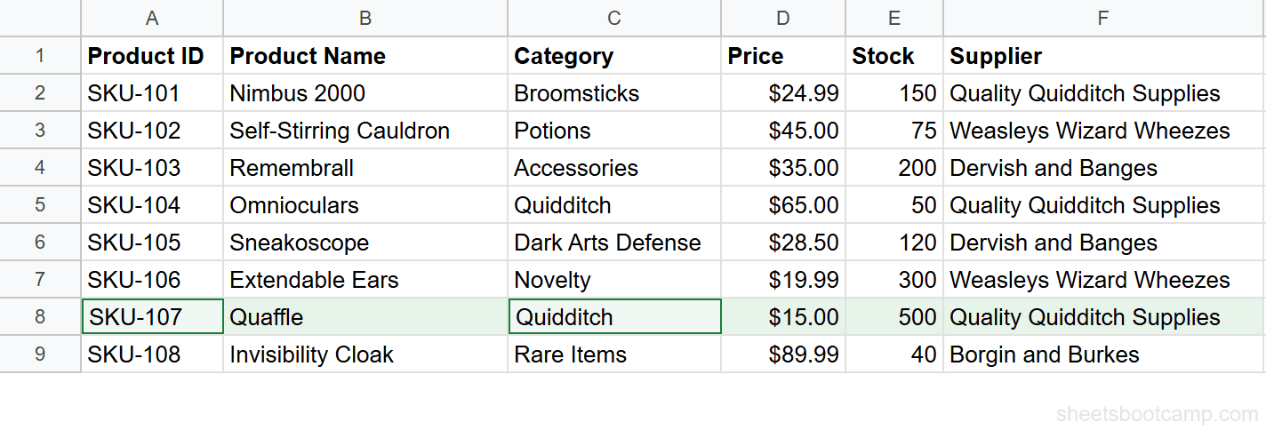
SKU-107 is the Quaffle, which is in the Quidditch category and priced at $15.00.
Build the condition arrays
Each condition produces an array of TRUE/FALSE values across 8 rows:
(A2:A9="SKU-107") → {F, F, F, F, F, F, T, F}
(C2:C9="Quidditch") → {F, F, F, T, F, F, T, F}
Multiplying them: {0, 0, 0, 0, 0, 0, 1, 0} — only row 7 (the Quaffle) has 1 because it matches both criteria.
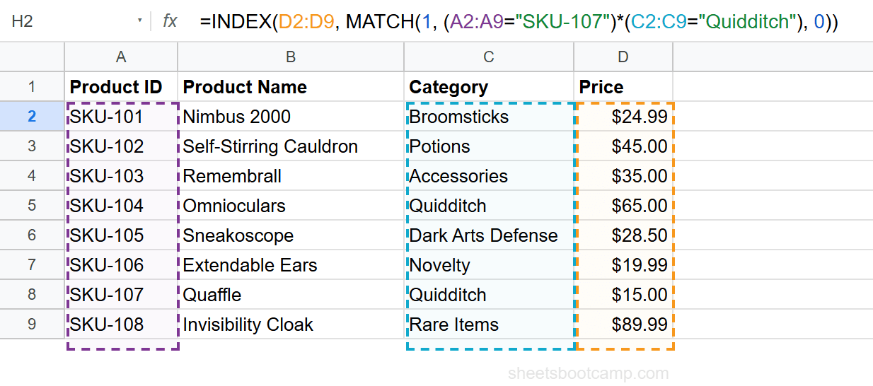
Write the full formula
=INDEX(D2:D9, MATCH(1, (A2:A9="SKU-107")*(C2:C9="Quidditch"), 0))- MATCH finds
1at position 7 in the multiplied array - INDEX returns the 7th value from D2:D9, which is $15.00
Test the condition arrays separately before combining them. Enter =MATCH(1, (A2:A9="SKU-107")*(C2:C9="Quidditch"), 0) by itself to confirm MATCH returns the correct position. Then wrap it in INDEX.
Practical Examples
Example 1: Find Stock by Category and Supplier
You want the stock count for Quidditch items supplied by Quality Quidditch Supplies:
=INDEX(E2:E9, MATCH(1, (C2:C9="Quidditch")*(F2:F9="Quality Quidditch Supplies"), 0))This returns 50 — the stock for Omnioculars (SKU-104), the first Quidditch product from Quality Quidditch Supplies.
Example 2: Find Product Name by Category and Price
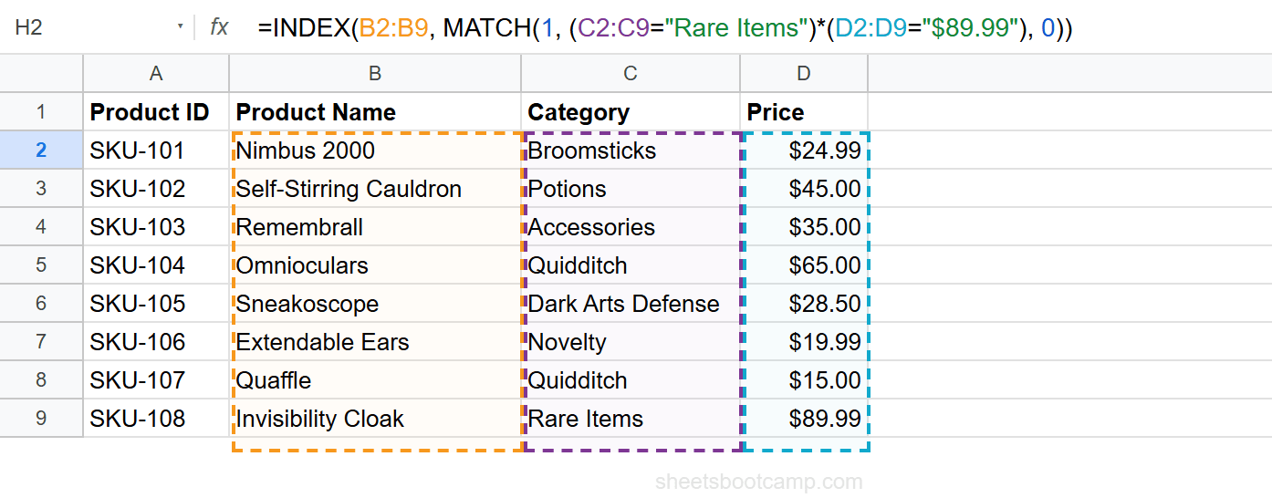
You want the product name for a Rare Items product priced at $89.99:
=INDEX(B2:B9, MATCH(1, (C2:C9="Rare Items")*(D2:D9="$89.99"), 0))This returns Invisibility Cloak (SKU-108). MATCH finds the row where both the category is “Rare Items” and the price is “$89.99”, and INDEX pulls the product name.
Example 3: Dynamic Criteria from Cells
Instead of hardcoding the criteria, reference cells. Place the Product ID in H2 and the Category in I2:
=INDEX(D2:D9, MATCH(1, (A2:A9=H2)*(C2:C9=I2), 0))Change the values in H2 and I2, and the formula updates automatically. This pattern works well with data validation dropdowns for interactive dashboards.
Three or More Criteria
Add more conditions by multiplying additional arrays. The pattern scales to any number of criteria.
Find the price for a Quidditch item from Quality Quidditch Supplies with stock above 100:
=INDEX(D2:D9, MATCH(1, (C2:C9="Quidditch")*(F2:F9="Quality Quidditch Supplies")*(E2:E9>100), 0))This checks three conditions:
- Category = “Quidditch”
- Supplier = “Quality Quidditch Supplies”
- Stock > 100
The only product matching all three is the Quaffle (SKU-107) with 500 in stock. The formula returns $15.00.
Each additional condition narrows the search. If no row matches all conditions, the formula returns #N/A. Wrap in IFERROR to handle this gracefully: =IFERROR(INDEX(..., MATCH(1, ..., 0)), "No match").
Compared to VLOOKUP with a Helper Column
VLOOKUP with multiple criteria requires a helper column that concatenates the criteria values. For example, to match on Product ID and Category, you would add a column with =A2&C2, then VLOOKUP against that concatenated column.
Helper column approach:
- Add a helper column with
=A2&C2in each row - VLOOKUP searches the helper column for “SKU-107Quidditch”
INDEX MATCH approach:
=INDEX(D2:D9, MATCH(1, (A2:A9="SKU-107")*(C2:C9="Quidditch"), 0))No helper column needed. The formula handles everything inline.
| Aspect | VLOOKUP + Helper Column | INDEX MATCH Array |
|---|---|---|
| Extra columns | Yes (one helper column) | None |
| Formula clarity | Easier to read (single VLOOKUP) | More complex formula |
| Data modification | Requires adding a column | No changes to data |
| Maintenance | Helper column must stay in sync | Self-contained |
| Conditions | Concatenation handles two; awkward beyond that | Scales to any number |
INDEX MATCH is the cleaner solution when you do not want to modify your data. The helper column approach is easier to audit because each step is visible in the sheet.
Common Errors
#N/A Error
No row matched all conditions. Common causes:
- Typo in a criteria value — “Quiditch” instead of “Quidditch”
- Extra spaces — “SKU-107 ” (trailing space) does not match “SKU-107”
- Different data types — searching for the number 107 in a column of text values
Fix: Verify each criterion matches the data. Use =TRIM() to clean whitespace. Check data types with =TYPE().
#VALUE! Error
The ranges in the condition arrays have different sizes. (A2:A9="SKU-107") has 8 rows, but (C2:C5="Quidditch") has only 4.
Fix: Make all ranges the same length. Every condition array and the INDEX return range should have the same number of rows.
Wrong Result
The formula returns a value, but it is from the wrong row. This happens when:
- The multiplication produces
1in an unexpected row because condition values overlap - You used
MATCH(0, ...)instead ofMATCH(1, ...)
Fix: Check your condition values against the data. Confirm you are searching for 1 (both conditions true), not 0.
If multiple rows match all criteria, MATCH returns the first match only. The formula does not return multiple results. If you need all matching rows, use the FILTER function instead.
Tips
-
Always search for 1, not TRUE. The multiplication converts TRUE/FALSE to 1/0. Use
MATCH(1, ...)to find the first row where all conditions are met. -
Use cell references for dynamic criteria. Replace hardcoded values with cell references:
(A2:A9=H2)*(C2:C9=I2). This makes the formula reusable and works with dropdown menus. -
Wrap in IFERROR for user-facing sheets.
=IFERROR(INDEX(..., MATCH(1, ..., 0)), "No match")prevents #N/A from appearing when the criteria combination does not exist. -
Test MATCH separately first. Before writing the full formula, test
=MATCH(1, (condition1)*(condition2), 0)alone to confirm it returns the expected position. -
Keep condition ranges consistent. All arrays in the multiplication must have the same number of rows. A mismatch causes #VALUE!.
Related Google Sheets Tutorials
- INDEX MATCH: The Complete Guide — Full syntax, left lookups, two-way lookups, and the combined formula pattern
- INDEX MATCH for Beginners — Start here if you are new to INDEX MATCH
- INDEX MATCH vs VLOOKUP — When to use each lookup formula
- VLOOKUP with Multiple Criteria — The helper column approach with VLOOKUP
- IF with AND / OR — Combine multiple conditions in IF formulas
Frequently Asked Questions
Can INDEX MATCH handle two conditions in Google Sheets?
Yes. Multiply two condition arrays inside MATCH and search for 1. The formula is =INDEX(return_range, MATCH(1, (condition1)*(condition2), 0)). This finds the first row where both conditions are true.
Do I need Ctrl+Shift+Enter for multi-criteria INDEX MATCH?
In current versions of Google Sheets, a regular Enter press works. Older versions may require Ctrl+Shift+Enter to enter the formula as an array. If the formula returns an error, try the Ctrl+Shift+Enter approach.
Can I use more than two criteria with INDEX MATCH?
Yes. Add more condition arrays multiplied together: (condition1)*(condition2)*(condition3). Each additional condition narrows the match. There is no fixed limit on the number of conditions.
Is multi-criteria INDEX MATCH better than VLOOKUP with a helper column?
INDEX MATCH handles multiple criteria in a single formula without modifying your data. The VLOOKUP approach requires adding a helper column that concatenates the criteria. INDEX MATCH is cleaner, but the helper column approach is easier to audit.
Why does my multi-criteria INDEX MATCH return #N/A?
The #N/A error means no row matched all conditions. Check that the values exist in the data, watch for extra spaces or case differences, and verify you are searching the correct columns. Use MATCH(1, ...) not MATCH(0, ...).