INDIRECT Function in Google Sheets (Dynamic References)
Learn how to use the INDIRECT function in Google Sheets to create dynamic cell references. Covers syntax, examples with data validation, and common errors.
Sheets Bootcamp
June 19, 2026
The INDIRECT function in Google Sheets converts a text string into a cell reference, letting you build references that change dynamically based on other cell values. It’s the key to creating formulas that adapt — pointing at different sheets, ranges, or cells without editing the formula itself.
This guide covers the INDIRECT syntax, step-by-step examples with dropdowns and cross-sheet references, and how to fix the #REF! errors that come up most often.
In This Guide
- What Is the INDIRECT Function?
- Syntax and Parameters
- How to Use INDIRECT: Step-by-Step
- INDIRECT Examples
- Common Errors and How to Fix Them
- Tips and Best Practices
- Related Google Sheets Tutorials
- FAQ
What Is the INDIRECT Function?
INDIRECT takes a text string and interprets it as a cell reference. You give it "A1" as text, and it returns whatever value lives in cell A1. On its own, that’s not useful — you could reference A1 directly. The function becomes valuable when the text string is built from other cells.
For example, if a dropdown in B1 contains a sheet tab name, =INDIRECT(B1&"!A1") pulls the value from cell A1 on whichever sheet the user selects. Change the dropdown, and the formula points somewhere new. This is how dependent dropdowns and dynamic dashboards work behind the scenes.
Syntax and Parameters
=INDIRECT(cell_reference_as_string, [is_A1_notation])| Parameter | Description | Required |
|---|---|---|
| cell_reference_as_string | A text string that represents a cell or range reference (e.g., "A1", "Sheet2!B5", "A1:C10") | Yes |
| is_A1_notation | TRUE (default) for A1 notation. FALSE for R1C1 notation | No |
INDIRECT only accepts text strings. Passing a direct cell reference like =INDIRECT(A1) reads the text value stored in A1 and interprets that as a reference. It does not reference A1 itself.
How to Use INDIRECT: Step-by-Step
We’ll build a formula that pulls data from different sheet tabs based on a dropdown selection.
Build a reference string
Set up a dropdown in cell B1 with the names of your sheet tabs (e.g., “January”, “February”, “March”). Each tab contains monthly sales data in the same layout with totals in cell D2.
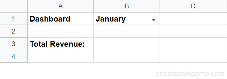
Enter the INDIRECT formula
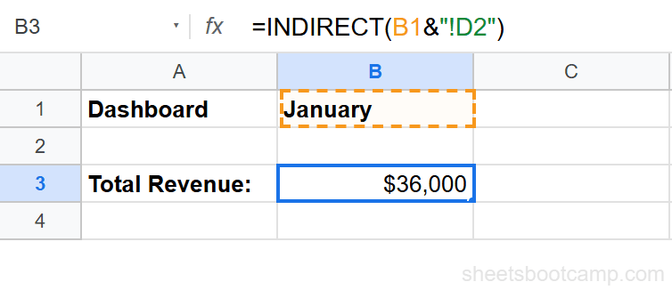
Click cell B3 and enter the formula that combines the dropdown value with the cell address:
=INDIRECT(B1&"!D2")This concatenates the sheet name in B1 (e.g., “January”) with "!D2" to form "January!D2", which INDIRECT interprets as a reference to cell D2 on the January tab.
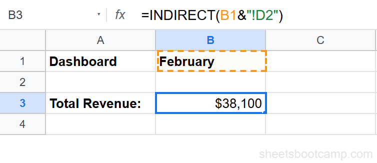
Verify the dynamic result
Change the dropdown in B1 from “January” to “February.” The INDIRECT formula automatically returns the value from cell D2 on the February tab — no formula editing needed.
If your tab names contain spaces (like “Q1 Sales”), wrap them in single quotes inside the formula: =INDIRECT("'"&B1&"'!D2").
INDIRECT Examples
Reference a Cell Based on Row Number
Build a dynamic reference where the row number comes from another cell. If cell A1 contains the number 5:
=INDIRECT("B"&A1)This creates the reference "B5" and returns the value in cell B5. Change A1 to 10, and the formula returns the value in B10.
Use INDIRECT with VLOOKUP Across Sheets
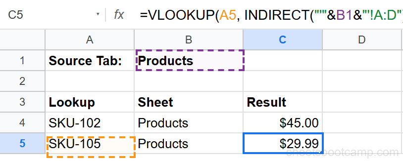
Let a dropdown control which sheet VLOOKUP searches. With a sheet name in B1:
=VLOOKUP(A5, INDIRECT("'"&B1&"'!A:D"), 3, FALSE)This searches columns A through D on whichever sheet B1 points to. Changing B1 switches the lookup table without modifying the formula.
Build a Named Range Reference Dynamically
If you have named ranges like “Sales_Q1”, “Sales_Q2”, etc., INDIRECT can reference them by name:
=SUM(INDIRECT("Sales_"&C1))When C1 contains “Q1”, this evaluates to =SUM(Sales_Q1). Change C1 to “Q2” and it sums the Q2 range instead.
Common Errors and How to Fix Them
#REF! Error
The text string doesn’t resolve to a valid reference. This is the most common INDIRECT error. Check for:
- Misspelled sheet names in the source cell
- Missing exclamation mark between the sheet name and cell address
- Sheet names with spaces that aren’t wrapped in single quotes
#VALUE! Error
The cell_reference_as_string argument is empty or contains a value that can’t be interpreted as a reference. Verify the source cell isn’t blank and contains a properly formatted reference string.
Circular Reference Error
INDIRECT references the cell it’s in, or references a cell that refers back to it. Restructure the formula so the reference string doesn’t create a loop.
Use =FORMULATEXT(B3) to see the text string INDIRECT is actually receiving. This helps debug complex concatenations where the assembled reference might not match what you expect.
Tips and Best Practices
-
Handle tab names with spaces. Wrap the sheet name in single quotes inside your concatenation:
=INDIRECT("'"&B1&"'!A1"). Without the quotes, Sheets can’t parse the reference. -
Pair INDIRECT with data validation. Dropdowns make INDIRECT formulas user-friendly. The person using the sheet picks from a list, and the formula handles the rest.
-
Watch for performance impact. INDIRECT is a volatile function — it recalculates on every change, even when its inputs haven’t changed. In sheets with thousands of INDIRECT formulas, consider replacing them with INDEX MATCH where possible.
-
Use named ranges for readability.
=INDIRECT("totals_"&B1)is easier to read and maintain than=INDIRECT("'"&B1&"'!D"&MATCH("Total",A:A,0)). Set up named ranges on each tab to keep INDIRECT formulas clean. -
INDIRECT references don’t update when you rename sheets. Unlike direct references, INDIRECT references are text strings. If you rename a tab from “January” to “Jan”, formulas referencing “January” break. Update the source cells or dropdown values to match.
Related Google Sheets Tutorials
- Named Ranges in Google Sheets - Create named ranges that INDIRECT can reference dynamically
- Dependent Drop-Down Lists in Google Sheets - Build cascading dropdowns powered by INDIRECT
- VLOOKUP: The Complete Guide - Combine VLOOKUP with INDIRECT for cross-sheet lookups
- INDEX MATCH in Google Sheets - A non-volatile alternative for dynamic lookups
FAQ
What does the INDIRECT function do in Google Sheets?
INDIRECT converts a text string into a cell reference. You pass it a string like "A1" or "Sheet2!B5" and it returns the value at that address. This lets you build references dynamically using other cell values.
How do I use INDIRECT to reference another sheet?
Concatenate the sheet name with the cell address: =INDIRECT("Sheet2!A1"). If the sheet name comes from a cell, use =INDIRECT(A1&"!B2") where A1 contains the sheet name. Wrap sheet names with spaces in single quotes: =INDIRECT("'"&A1&"'!B2").
Can I use INDIRECT with VLOOKUP?
Yes. Use INDIRECT to build the VLOOKUP table range dynamically: =VLOOKUP(A2, INDIRECT("'"&B1&"'!A:C"), 2, FALSE). This lets you switch which sheet VLOOKUP searches by changing a single cell value.
Why does INDIRECT return a #REF! error?
The text string doesn’t resolve to a valid cell reference. Check for typos in the sheet name, missing exclamation marks, or sheet names with spaces that need single quotes. Also verify the referenced sheet exists in the spreadsheet.
Is INDIRECT volatile in Google Sheets?
Yes. INDIRECT recalculates every time the spreadsheet recalculates, even if its inputs haven’t changed. In large spreadsheets with hundreds of INDIRECT formulas, this can slow performance. Use direct references when the target doesn’t need to change dynamically.
What is the difference between INDIRECT and direct cell references?
A direct reference like =A1 is fixed in the formula. INDIRECT("A1") interprets the text string "A1" as a reference at runtime. The advantage is that you can change the target by changing the text string, which enables dynamic formulas driven by dropdowns or other inputs.