MAX, MIN, LARGE, SMALL in Google Sheets
Learn how to use MAX, MIN, LARGE, and SMALL functions in Google Sheets. Find the highest, lowest, and nth-ranked values in any range.
Sheets Bootcamp
March 7, 2026 · Updated June 18, 2026
MAX and MIN find the highest and lowest values in a range. LARGE and SMALL extend this by letting you find the 2nd highest, 3rd lowest, or any specific rank in your data. These four functions are the foundation for finding extremes and building top-N reports in Google Sheets.
This guide covers all four functions: MAX and MIN for absolute extremes, LARGE and SMALL for ranked values, and practical combinations for real-world use.
In This Guide
- When to Use Each Function
- Syntax and Parameters
- How to Use MAX, MIN, LARGE, SMALL: Step-by-Step
- Practical Examples
- Common Errors and How to Fix Them
- Tips and Best Practices
- Related Google Sheets Tutorials
- FAQ
When to Use Each Function
| Function | Returns | Example |
|---|---|---|
| MAX | The largest value | Highest revenue in a quarter |
| MIN | The smallest value | Lowest test score in a class |
| LARGE | The nth largest value | The 3rd highest salary |
| SMALL | The nth smallest value | The 2nd lowest price |
MAX and MIN give you the absolute extremes. LARGE and SMALL let you pick any rank in between.
Syntax and Parameters
MAX / MIN
=MAX(value1, [value2], ...)=MIN(value1, [value2], ...)| Parameter | Description | Required |
|---|---|---|
| value1 | A number, cell reference, or range | Yes |
| value2 | Additional values or ranges | No |
LARGE / SMALL
=LARGE(data, n)=SMALL(data, n)| Parameter | Description | Required |
|---|---|---|
| data | The range of numeric values | Yes |
| n | The rank to return (1 = largest/smallest, 2 = second, etc.) | Yes |
LARGE(data, 1) equals MAX(data) and SMALL(data, 1) equals MIN(data). If n is larger than the number of values in the range, the function returns a #NUM! error.
How to Use MAX, MIN, LARGE, SMALL: Step-by-Step
We’ll find the highest, lowest, and top-3 revenue values from a sales dataset.
Identify your numeric range
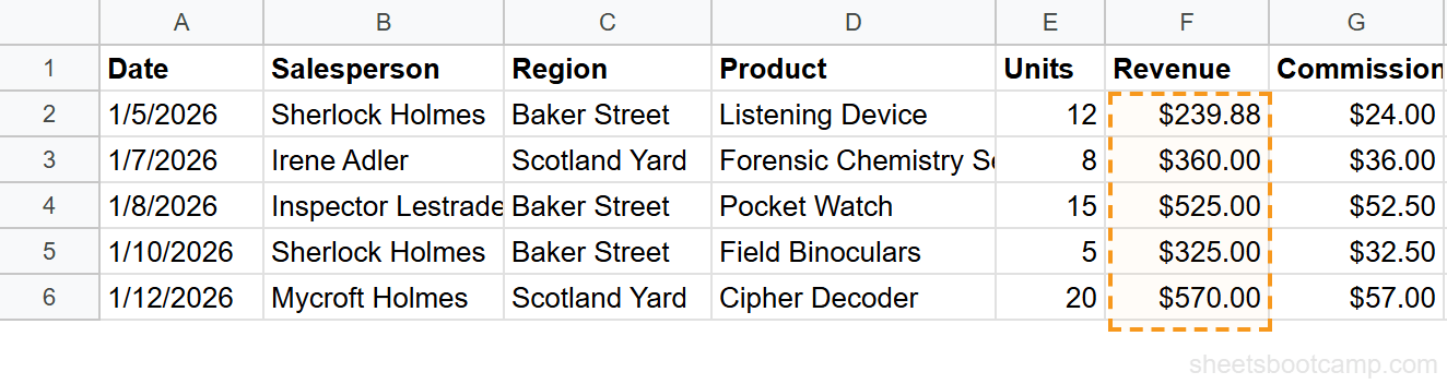
The sales data has 18 rows with Revenue values in column F. These are the numbers we want to analyze.
Enter the MAX and MIN formulas
In separate cells, enter both formulas:
=MAX(F2:F19)=MIN(F2:F19)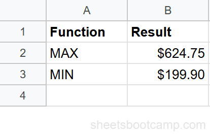
MAX returns $624.75 (Irene Adler’s Magnifying Glass sale). MIN returns $199.90 (Inspector Lestrade’s Listening Device sale).
Use LARGE for ranked values
Find the top 3 revenue values:
=LARGE(F2:F19, 1)=LARGE(F2:F19, 2)=LARGE(F2:F19, 3)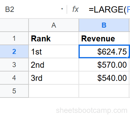
To build a dynamic top-N list, use LARGE with row numbers: put 1, 2, 3 in a column, then reference those cells in the LARGE formula. Adding a new row automatically extends the ranking.
Practical Examples
Find Who Had the Highest Sale
Combine MAX with INDEX MATCH to find who made the largest sale:
=INDEX(B2:B19, MATCH(MAX(F2:F19), F2:F19, 0))MAX finds the highest revenue ($624.75), MATCH locates its row position, and INDEX returns the corresponding salesperson name from column B.
Range (Difference Between Max and Min)
Calculate the spread of values:
=MAX(F2:F19) - MIN(F2:F19)This returns the range — the difference between the highest and lowest values. Useful for measuring variability in a dataset.
Top 3 with Corresponding Names
Use LARGE and INDEX MATCH together to build a leaderboard:
=INDEX(B2:B19, MATCH(LARGE(F2:F19, 1), F2:F19, 0))Change the LARGE rank (1, 2, 3) to get the names for the top three performers. This powers dashboard-style top-N displays.
Conditional MAX (Highest in a Group)
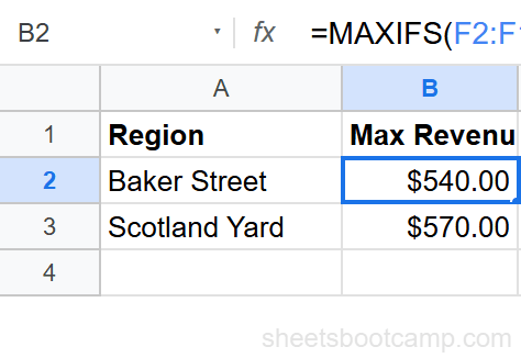
Find the highest revenue in a specific region using MAXIFS:
=MAXIFS(F2:F19, C2:C19, "Baker Street")MAXIFS works like MAX but with conditions. MINIFS does the same for the minimum. These are available natively in Google Sheets.
Second Lowest Price
Find the second cheapest product in a price list:
=SMALL(D2:D12, 2)SMALL with n=2 skips the absolute minimum and returns the next lowest value. Useful for excluding outliers or finding runner-up values.
Common Errors and How to Fix Them
#NUM! Error
The n argument in LARGE or SMALL exceeds the number of values in the range. If you have 18 values, =LARGE(F2:F19, 20) returns #NUM! because there is no 20th value. Reduce n to match or stay within the data count.
Returns 0 Instead of Expected Value
The range contains no numeric values, or all cells are blank/text. MAX and MIN return 0 when there’s nothing to evaluate. Check that your cells contain actual numbers (not text formatted to look like numbers).
MAX and MIN return 0 for empty ranges, not an error. This can cause misleading results in reports. Use =IF(COUNT(F2:F19)>0, MAX(F2:F19), “No data”) to handle empty ranges explicitly.
Wrong Result with Dates
Dates in Google Sheets are numbers. MAX on a date column returns the most recent date (largest serial number). MIN returns the earliest date. This is correct behavior, but format the result cell as a date so it displays properly instead of showing a serial number.
Tips and Best Practices
-
Use MAXIFS and MINIFS for conditional extremes.
=MAXIFS(F2:F19, C2:C19, "Scotland Yard")finds the highest value in a specific group. These functions work like SUMIF but for max/min. -
Build top-N reports with LARGE. Create a column of ranks (1, 2, 3, 4, 5) and reference them in LARGE formulas. Pair with INDEX MATCH to pull corresponding details like names or dates.
-
Combine with conditional formatting to highlight extremes. Set a rule to highlight the cell equal to MAX(range) in green and MIN(range) in red. The highlights update automatically as values change.
-
MAX and MIN work across multiple ranges. =MAX(A2:A10, C2:C10, E2:E10) finds the highest value across three separate columns in one formula.
-
Use SMALL to exclude outliers. If your minimum is an obvious data entry error, use SMALL(range, 2) to find the “real” minimum while ignoring the lowest outlier.
Related Google Sheets Tutorials
- AVERAGE, AVERAGEIF, and AVERAGEIFS - Calculate means alongside max/min for statistical analysis
- COUNT, COUNTA, COUNTBLANK - Count cells by type to validate your data before finding extremes
- SORT Function in Google Sheets - Sort data by value to see the ranking visually
- INDEX MATCH in Google Sheets - Look up the name or detail that corresponds to a MAX or MIN value
FAQ
How do I find the highest value in Google Sheets?
Use =MAX(range). For example, =MAX(B2:B100) returns the largest number in the range. MAX ignores text and blank cells.
How do I find the lowest value in Google Sheets?
Use =MIN(range). For example, =MIN(B2:B100) returns the smallest number in the range. MIN ignores text and blank cells.
How do I find the 2nd or 3rd highest value?
Use =LARGE(range, n) where n is the rank. =LARGE(B2:B100, 2) returns the second highest value, =LARGE(B2:B100, 3) returns the third highest, and so on. LARGE(range, 1) is the same as MAX(range).
What is the difference between MAX and LARGE?
MAX always returns the single highest value. LARGE returns the nth highest value based on the rank you specify. MAX(range) equals LARGE(range, 1). Use LARGE when you need the top 2, top 3, or any specific rank.
Do MAX and MIN ignore text and blanks?
Yes. MAX, MIN, LARGE, and SMALL all ignore text, blank cells, and logical values (TRUE/FALSE). They only evaluate numeric values. If the range has no numbers, they return 0.
How do I find the top 5 values in Google Sheets?
Use LARGE with an array: enter =LARGE(F2:F19, 1) through =LARGE(F2:F19, 5) in five cells. Or use =LARGE(F2:F19, ROW(1:5)) as an array formula to output all five values at once.