Custom Number Formats in Google Sheets (Guide)

Custom number formats in Google Sheets control how numbers display without changing the underlying values. The number 36000 can show as $36,000.00, 36K, or 3.6E+04 — the cell still holds 36000 for calculations.

This guide covers the built-in format options, custom format codes for currency, percentages, dates, and conditional colors, and how to build multi-section formats that handle positive, negative, and zero values differently.

In This Guide

• What Are Custom Number Formats?
• Syntax and Parameters
• How to Apply Custom Number Formats: Step-by-Step
• Number Format Examples
• Common Errors and How to Fix Them
• Tips and Best Practices
• Related Google Sheets Tutorials
• FAQ

What Are Custom Number Formats?

Google Sheets separates what a cell contains from how it appears. A cell might hold the value 0.15, but you can display it as 15%, $0.15, or 0.2 (rounded). Custom number formats give you control over the display without touching the underlying data.

This matters because formulas always use the stored value, not the displayed one. Format a cell as currency and it still calculates like a regular number.

Syntax and Parameters

Custom number format codes use placeholder characters to define the display. Here are the building blocks:

Multi-Section Formats

Separate up to four sections with semicolons to handle different value types:

positive;negative;zero;text

Example: $#,##0.00;[Red]-$#,##0.00;$0.00;"Text: "@

How to Apply Custom Number Formats: Step-by-Step

We’ll format a column of revenue numbers as currency with thousands separators.

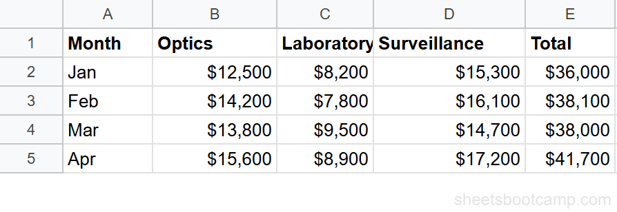
Highlight column E (Total) in the monthly summary data, which contains raw numbers like 36000, 38100, and 38000.

Go to Format > Number > Custom number format. In the text field, type the format code:

$#,##0

This displays numbers with a dollar sign, thousands separators, and no decimal places.

Click Apply. The value 36000 now displays as $36,000. The underlying value hasn’t changed — select the cell and the formula bar still shows 36000.

Number Format Examples

Currency with Two Decimal Places

$#,##0.00

Displays 1500.5 as $1,500.50. The 0.00 forces two decimal places. Use $#,##0 to drop the cents.

Percentage with One Decimal

0.0%

Displays 0.156 as 15.6%. Remember, the cell must contain the decimal value (0.156), not the whole number (15.6).

Negative Numbers in Red

$#,##0.00;[Red]-$#,##0.00

Positive values display as $1,500.00 in default black text. Negative values display as -$1,500.00 in red. Available color codes: [Red], [Blue], [Green], [Yellow], [Magenta], [Cyan], [White], [Black].

Thousands Abbreviation (K)

#,##0.0,"K"

Displays 36000 as 36.0K. The comma before “K” divides the value by 1,000 for display purposes. Add two commas for millions: #,##0.0,,"M" shows 1500000 as 1.5M.

Add Units or Labels

#,##0" units"

Displays 500 as 500 units. Text inside double quotes appears as-is. The cell still holds 500, so =A1*2 returns 1000.

Date Formats

yyyy-mm-dd

Displays a date serial number as 2026-06-24. Other patterns: mm/dd/yyyy for 06/24/2026, mmm d, yyyy for Jun 24, 2026, dddd, mmmm d for Wednesday, June 24.

For more date formatting options, see the Format Dates guide.

Common Errors and How to Fix Them

Numbers Show as Text

The cell contains a text string that looks like a number, not an actual number. The green triangle in the top-left corner is the clue. Click the cell, then click the warning icon and select “Convert to number.” Formatting only affects actual numeric values.

Percentage Shows 1500% Instead of 15%

The cell contains 15 instead of 0.15. The % format multiplies the stored value by 100. Enter 0.15 to see 15%. If you already have whole numbers, use the format #,##0"%" (with quotes around %) to add a percent symbol without multiplying.

Decimals Appear to Be Rounded

The format code is hiding decimal places, not rounding the stored value. $#,##0 displays 1500.75 as $1,501 (visually rounded), but the cell still contains 1500.75. Calculations use the full value. If you need the actual value rounded, use the ROUND function.

Tips and Best Practices

1. Format columns, not individual cells. Select the entire column before applying a format so new data entered below inherits the same display rules.

2. Use built-in formats first. Format > Number offers Currency, Percent, Date, and other presets. Only go to Custom number format when the presets don’t match what you need.

3. Don’t confuse formatting with data. If you need to display “15%” and calculate with 15, use the format #,##0"%" (quotes around the percent). Without quotes, 0% treats 15 as 1500%.

4. Combine with conditional formatting for visual rules. Number formats control display; conditional formatting controls color based on values. Use both: format as currency, then highlight values above $50,000 in green.

5. Test with edge cases. Apply your format to 0, a negative number, a large number, and a small decimal. Multi-section formats (positive;negative;zero) let you handle each case differently.

Related Google Sheets Tutorials

• Format Dates in Google Sheets - Custom date format codes for displaying dates in any layout
• Conditional Formatting: The Complete Guide - Apply colors and icons based on cell values alongside number formats
• Text Functions in Google Sheets - Convert formatted numbers to text or extract numeric parts from strings
• Absolute vs Relative References - Understand cell references before applying formatting to formula results

FAQ

How do I create a custom number format in Google Sheets?

Go to Format > Number > Custom number format. Type your format code in the text field and click Apply. Common codes: # for optional digits, 0 for required digits, . for decimal point, , for thousands separator, $ for currency symbol.

What does the # symbol mean in number formats?

The # symbol represents an optional digit placeholder. It displays a digit if there is one, but shows nothing if the position is empty. For example, #,##0 displays 1000 as 1,000 and 50 as 50 (not 050).

How do I format numbers as currency in Google Sheets?

Select the cells, then press Ctrl+Shift+4 (or Cmd+Shift+4 on Mac) for quick currency format. For custom currency, go to Format > Number > Custom number format and type $#,##0.00 for dollars with cents, or $#,##0 for dollars without cents.

How do I show negative numbers in red?

Use a two-section format: $#,##0.00;[Red]-$#,##0.00. The semicolon separates the positive format from the negative format. The [Red] color code makes negative values display in red text.

Can I add text to a number format?

Yes. Wrap text in double quotes inside the format code. For example, #,##0" units" displays 500 as 500 units. The underlying value stays 500, so formulas still work with the raw number.

What is the difference between formatting and changing a value?

Formatting changes how a number displays without changing the number itself. The value 0.15 formatted as a percentage shows 15%, but the cell still contains 0.15. Formulas reference the underlying value, not the displayed format.