Pivot Tables in Google Sheets: Beginner's Guide

A pivot table in Google Sheets summarizes large datasets into compact, readable tables. You pick the columns to group by and the values to aggregate, and Sheets builds the summary for you. No formulas required.

This guide walks you through creating your first pivot table, changing summary functions, adding multiple dimensions, and filtering results. Every example uses real data so you can follow along.

In This Guide

• What Is a Pivot Table?
• How to Create a Pivot Table: Step-by-Step
• Pivot Table Examples
• How to Edit and Update a Pivot Table
• Tips and Best Practices
• Common Pivot Table Problems and Fixes
• Related Google Sheets Tutorials
• FAQ

What Is a Pivot Table?

A pivot table takes a flat list of records and groups them by one or more categories. It then applies a function (SUM, COUNT, AVERAGE, or others) to summarize the values in each group. The name comes from “pivoting” your data — rotating it from a long list into a compact summary.

Here is when you would use one:

• You have a list of transactions and want total revenue by salesperson
• You need to count how many orders each region placed
• You want to compare average revenue across products

Pivot tables work through a visual editor. You drag fields into four areas: Rows (categories down the left side), Columns (categories across the top), Values (the numbers to summarize), and Filters (conditions to narrow the data). Google Sheets handles the math.

How to Create a Pivot Table: Step-by-Step

We’ll use a sales records table with 18 transactions. Each row has a date, salesperson, region, product, units, revenue, and commission.

Your data needs headers in row 1 and no blank rows or columns in the middle. Each column should contain one type of data (text, numbers, or dates).

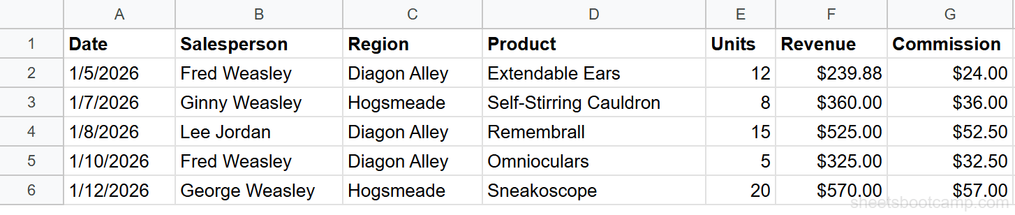
The sales records table has seven columns: Date, Salesperson, Region, Product, Units, Revenue, and Commission. All 18 rows are filled with consistent data.

Select any cell inside your data table. Go to Insert > Pivot table. Google Sheets detects the full data range automatically.

In the dialog that appears, you’ll see the data range pre-filled (for example, Sheet1!A1:G19). Choose New sheet to place the pivot table on its own tab. Click Create.

Google Sheets opens a new sheet with an empty pivot table and the Pivot table editor panel on the right side.

In the pivot table editor:

1. Next to Rows, click Add and select Salesperson
2. Next to Values, click Add and select Revenue

Google Sheets defaults to SUM for numeric columns. Each salesperson’s total revenue appears in the pivot table.

The finished pivot table shows one row per salesperson with their total revenue:

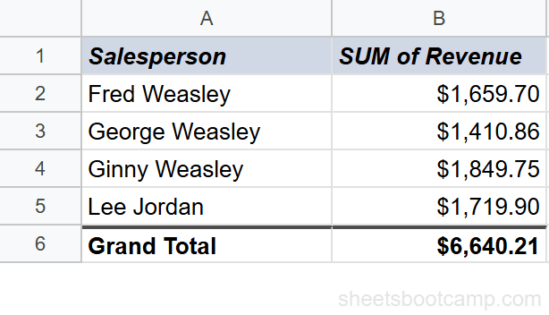
Ginny Weasley leads with $1,849.75 in total revenue. The grand total across all salespeople is $6,640.21. Google Sheets added the Grand Total row automatically.

Pivot Table Examples

Example 1: Revenue by Region (SUM)

To see revenue broken down by region instead of salesperson, create a new pivot table (or modify the existing one). Add Region to Rows and Revenue to Values.

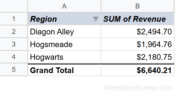
Diagon Alley generated $2,494.70, Hogsmeade $1,964.76, and Hogwarts $2,180.75.

Example 2: Number of Sales by Salesperson (COUNTA)

Change the Values function to count transactions instead of summing revenue. Add Salesperson to Rows and Date to Values. Then click the Summarize by dropdown under Values and select COUNTA (which counts non-empty cells).

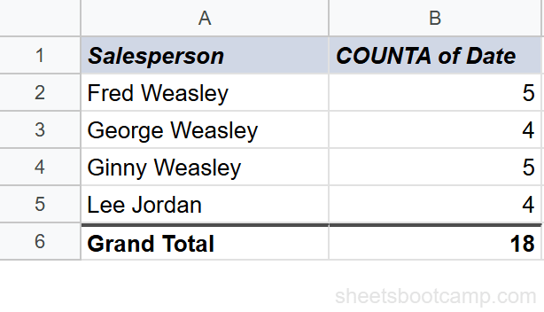
Fred Weasley and Ginny Weasley each made 5 sales. George Weasley and Lee Jordan each made 4. The total is 18 transactions.

Example 3: Average Revenue by Product (AVERAGE)

Add Product to Rows and Revenue to Values. Change Summarize by to AVERAGE. Sort the pivot table by average revenue descending to see the highest-value products first.

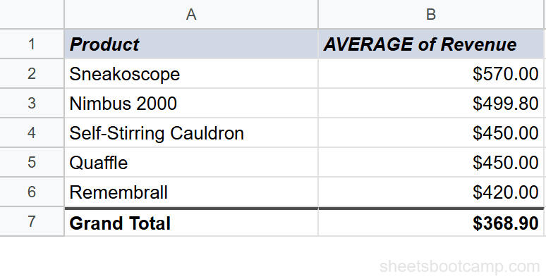
Sneakoscope has the highest average revenue at $570.00 (one transaction). Nimbus 2000 averages $499.80 across two transactions.

Example 4: Two Dimensions (Salesperson + Region)

Add Salesperson to Rows first, then add Region to Rows below it. Add Revenue as the Value (SUM). This creates a grouped layout where each salesperson shows a breakdown by region, with subtotals per salesperson and a grand total at the bottom.

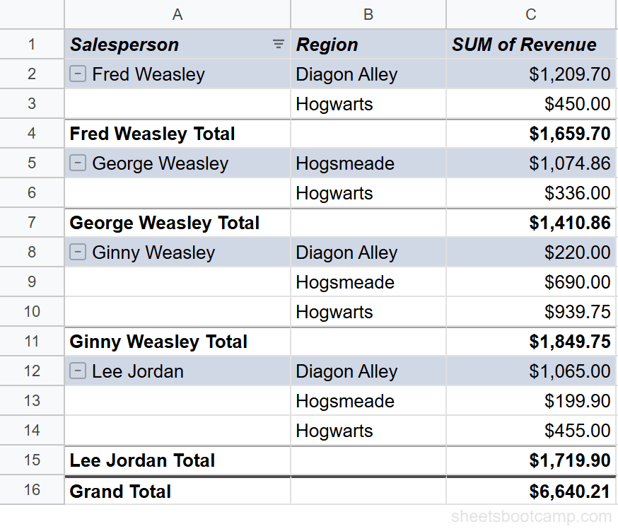
Fred Weasley sold $1,209.70 in Diagon Alley and $450.00 in Hogwarts, totaling $1,659.70. Each salesperson group has a collapse icon (−) that hides or shows the region breakdown. The group header rows have a blue tinted background to separate them visually from the detail rows.

How to Edit and Update a Pivot Table

Change the summary function

Click the Summarize by dropdown under any Value field in the pivot table editor. Options include SUM, COUNTA, AVERAGE, MAX, MIN, MEDIAN, and more. Switch from SUM to AVERAGE to see per-transaction averages instead of totals.

Add or remove fields

Click the X next to any field in the pivot table editor to remove it. Click Add to bring in a new field. You can have multiple fields in Rows, Columns, or Values at the same time.

Filter the pivot table

Click Add next to Filters in the pivot table editor. Select the column you want to filter by (for example, Region). Uncheck the values you want to exclude.

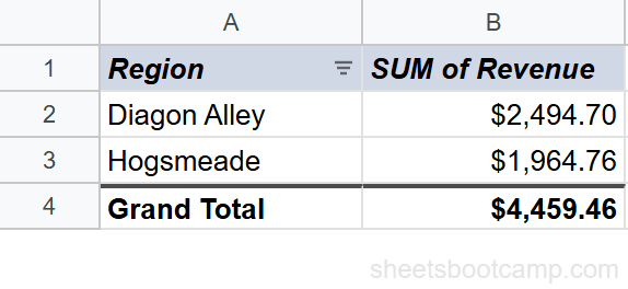
Filtering by Region with only Diagon Alley and Hogsmeade selected shows a combined total of $4,459.46. Hogwarts data is excluded from the summary.

Sort pivot table results

Click the Sort by dropdown in the Rows section of the pivot table editor. Choose the column to sort by and the direction (ascending or descending). Sorting by SUM of Revenue descending puts the highest-revenue salesperson at the top.

Tips and Best Practices

1. Clean your data first. Remove blank rows, merge duplicate headers, and make sure each column has consistent formatting. A pivot table is only as good as the data behind it.

2. Pivot tables refresh automatically. When you change values in the source data, the pivot table recalculates immediately. If you add new rows beyond the original range, update the data range in the pivot table by clicking the range reference at the top of the editor.

3. Use filters to focus on subsets. Instead of building separate pivot tables for each region, use the filter section to toggle between views of the same data.

4. Name your pivot table sheet. Double-click the sheet tab and rename it from “Pivot Table 1” to something descriptive like “Revenue by Region.” This makes it easier to find when your workbook grows.

5. Use the QUERY function for formula-based summaries. If you need a pivot-style summary that updates across sheets or feeds into other formulas, QUERY can produce similar output in a single formula.

Common Pivot Table Problems and Fixes

Blank rows in the pivot table

Cause: Blank rows or cells in your source data. The pivot table creates a separate group for blank values.

Fix: Go back to your source data and fill in or delete the blank rows. The pivot table updates automatically.

Wrong totals

Cause: Duplicate rows in the source data, or the data range includes extra rows with unrelated data.

Fix: Check the data range shown at the top of the pivot table editor. Make sure it covers only your actual data. Remove duplicates from the source using Data > Data cleanup > Remove duplicates.

Missing data

Cause: The pivot table’s data range does not include all rows. This happens when you add rows after creating the pivot table.

Fix: Click the data range at the top of the pivot table editor and expand it to include the new rows.

The pivot table editor disappeared

Cause: You clicked outside the pivot table area.

Fix: Click any cell inside the pivot table. The editor panel reappears on the right side.

Related Google Sheets Tutorials

• Google Sheets QUERY Function — Write formula-based summaries using SQL-like syntax
• SUMIF and SUMIFS — Sum values based on one or more conditions without a pivot table
• COUNTIF and COUNTIFS — Count entries that match specific criteria
• Google Sheets Charts — Visualize your pivot table results with bar charts, line charts, and pie charts

FAQ

What is a pivot table in Google Sheets?

A pivot table is a data summary tool that groups, counts, sums, or averages your data by category. You select which columns to use as rows, columns, values, and filters. Google Sheets builds the summary automatically.

How do I create a pivot table in Google Sheets?

Select any cell in your data, go to Insert > Pivot table, choose where to place it, and click Create. Then use the pivot table editor to add rows, columns, values, and filters.

Can I use multiple columns in a pivot table?

Yes. You can add multiple fields to rows, columns, and values. Adding Salesperson and Region to rows creates a grouped layout that shows revenue broken down by both dimensions with subtotals per group.

Does a pivot table update automatically?

Yes. When you change the source data, the pivot table recalculates automatically. If you add new rows outside the original range, you need to update the data range in the pivot table settings.

What is the difference between a pivot table and QUERY?

A pivot table uses a visual editor with drag-and-drop fields. The QUERY function uses a text-based query language inside a formula. Both can summarize data, but pivot tables are faster to set up and QUERY formulas are easier to reuse across sheets.