QUERY GROUP BY in Google Sheets (Summarize Data)
Learn how to use QUERY GROUP BY in Google Sheets to summarize data with SUM, COUNT, AVG, MIN, and MAX. Step-by-step examples and common mistakes.
Sheets Bootcamp
March 2, 2026
QUERY GROUP BY in Google Sheets collapses rows into groups and applies aggregate functions like SUM, COUNT, and AVG to each group. It turns a table of individual transactions into a summary report — one row per category, region, or person. It is one of the most useful clauses in the QUERY function and does the work of multiple SUMIF formulas in a single formula.
In This Guide
- GROUP BY Syntax
- How to Use GROUP BY: Step-by-Step
- Aggregate Functions Reference
- GROUP BY with Multiple Columns
- GROUP BY + WHERE (Filter Before Grouping)
- GROUP BY + ORDER BY (Sort the Summary)
- Rename Headers with LABEL
- Common Mistakes
- Tips
- Related Google Sheets Tutorials
- FAQ
GROUP BY Syntax
GROUP BY appears after WHERE (if used) in the query string:
=QUERY(data, "SELECT column, AGGREGATE(column) GROUP BY column")Every column in SELECT must either be in the GROUP BY clause or wrapped in an aggregate function. You cannot include a raw column that is not grouped or aggregated.
Every non-aggregated column in SELECT must appear in GROUP BY. SELECT B, SUM(F) GROUP BY C breaks because B is not grouped. Either change it to SELECT C, SUM(F) GROUP BY C or add B to GROUP BY.
How to Use GROUP BY: Step-by-Step
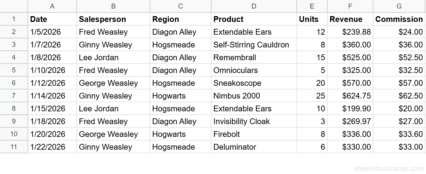
We’ll use the sales records table from the QUERY guide. The goal: total revenue by region.
Sample Data
| A | B | C | D | E | F | G | |
|---|---|---|---|---|---|---|---|
| 1 | Date | Salesperson | Region | Product | Units | Revenue | Commission |
| 2 | 1/5/2026 | Fred Weasley | Diagon Alley | Extendable Ears | 12 | $239.88 | $24.00 |
| 3 | 1/7/2026 | Ginny Weasley | Hogsmeade | Self-Stirring Cauldron | 8 | $360.00 | $36.00 |
| 4 | 1/8/2026 | Lee Jordan | Diagon Alley | Remembrall | 15 | $525.00 | $52.50 |
| 5 | 1/10/2026 | Fred Weasley | Diagon Alley | Omnioculars | 5 | $325.00 | $32.50 |
| 6 | 1/12/2026 | George Weasley | Hogsmeade | Sneakoscope | 20 | $570.00 | $57.00 |
| 7 | 1/14/2026 | Ginny Weasley | Hogwarts | Nimbus 2000 | 25 | $624.75 | $62.50 |
| 8 | 1/15/2026 | Lee Jordan | Hogsmeade | Extendable Ears | 10 | $199.90 | $20.00 |
| 9 | 1/18/2026 | Fred Weasley | Diagon Alley | Invisibility Cloak | 3 | $269.97 | $27.00 |
| 10 | 1/20/2026 | George Weasley | Hogwarts | Firebolt | 8 | $336.00 | $33.60 |
| 11 | 1/22/2026 | Ginny Weasley | Hogsmeade | Deluminator | 6 | $330.00 | $33.00 |
Review your data range
Your data is in A1:G11. Row 1 is the header. The Region column (C) has three unique values: Diagon Alley, Hogsmeade, and Hogwarts.
Write a GROUP BY query with SUM
Select an empty cell and enter:
=QUERY(A1:G11, "SELECT C, SUM(F) GROUP BY C")QUERY groups the 10 rows by Region and totals the Revenue for each group:
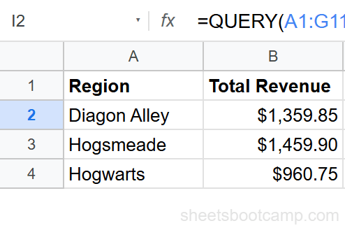
| Region | sum Revenue |
|---|---|
| Diagon Alley | $1,359.85 |
| Hogsmeade | $1,459.90 |
| Hogwarts | $960.75 |

Add a LABEL clause
The default header “sum Revenue” is not readable. Add LABEL to rename it:
=QUERY(A1:G11, "SELECT C, SUM(F) GROUP BY C LABEL SUM(F) 'Total Revenue'")The header now reads “Total Revenue” instead of “sum Revenue.”
Sort the results
Add ORDER BY to sort by total revenue, highest first:
=QUERY(A1:G11, "SELECT C, SUM(F) GROUP BY C ORDER BY SUM(F) DESC LABEL SUM(F) 'Total Revenue'")Hogsmeade ($1,459.90) now appears first, followed by Diagon Alley ($1,359.85) and Hogwarts ($960.75).
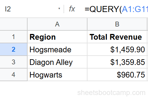
ORDER BY in a GROUP BY query sorts by the aggregated values, not the individual row values. ORDER BY SUM(F) DESC sorts regions by their total revenue, not by any single transaction.
Aggregate Functions Reference
| Function | What It Returns | Example |
|---|---|---|
SUM(col) | Total of all values | SUM(F) — total revenue |
COUNT(col) | Number of non-empty cells | COUNT(D) — number of transactions |
AVG(col) | Arithmetic average | AVG(F) — average revenue per transaction |
MIN(col) | Smallest value | MIN(F) — lowest revenue |
MAX(col) | Largest value | MAX(F) — highest revenue |
Multiple Aggregations
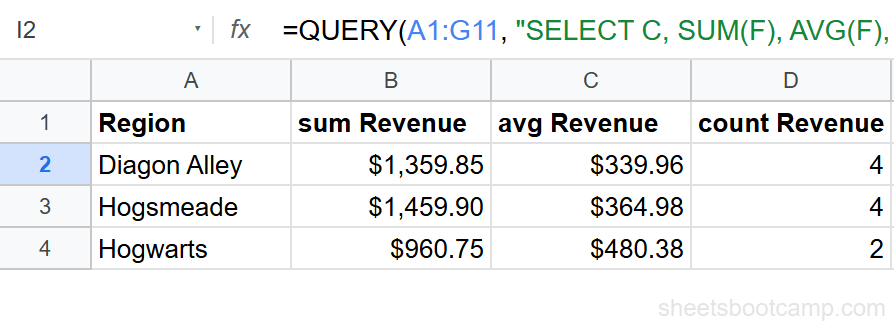
You can include multiple aggregate functions in a single SELECT:
=QUERY(A1:G11, "SELECT C, SUM(F), AVG(F), COUNT(F) GROUP BY C")This returns a summary table with total revenue, average revenue, and transaction count per region — all in one formula.
COUNT Example
=QUERY(A1:G11, "SELECT B, COUNT(D) GROUP BY B LABEL COUNT(D) 'Sales Count'")This counts transactions per salesperson. Fred Weasley: 3. Ginny Weasley: 3. George Weasley: 2. Lee Jordan: 2.
AVG Example
=QUERY(A1:G11, "SELECT C, AVG(F) GROUP BY C LABEL AVG(F) 'Avg Revenue'")This returns the average revenue per transaction for each region.
GROUP BY with Multiple Columns
GROUP BY accepts multiple columns separated by commas. This creates one row for each unique combination:
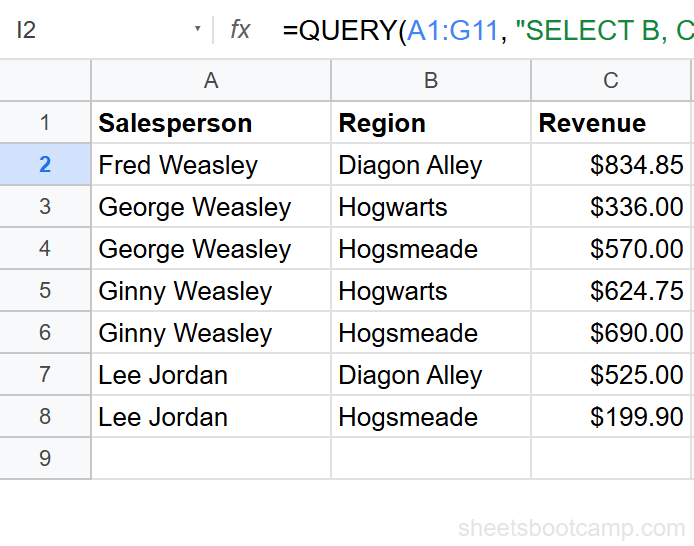
=QUERY(A1:G11, "SELECT B, C, SUM(F) GROUP BY B, C LABEL SUM(F) 'Revenue'")This groups by both Salesperson and Region. Fred Weasley in Diagon Alley gets his own row ($834.85). George Weasley in Hogsmeade gets a separate row ($570.00). Each unique pair is its own group.
Grouping by multiple columns increases the number of rows in the result. Grouping by Region alone gives 3 rows. Grouping by Salesperson and Region gives up to 12 rows (4 people times 3 regions), though only combinations that exist in the data appear.
GROUP BY + WHERE (Filter Before Grouping)
WHERE runs before GROUP BY. Use it to exclude rows before they get summarized:
=QUERY(A1:G11, "SELECT C, SUM(F) WHERE F > 300 GROUP BY C LABEL SUM(F) 'Revenue (>$300)'")This first filters out transactions under $300, then groups the remaining rows by region. The totals are lower because small transactions are excluded.
| Region | Revenue (>$300) |
|---|---|
| Diagon Alley | $850.00 |
| Hogsmeade | $1,260.00 |
| Hogwarts | $960.75 |
Only transactions over $300 are included in each total. Diagon Alley drops from $1,359.85 to $850.00 because two transactions ($239.88 and $269.97) are under the $300 threshold.
The WHERE clause guide covers all filter types — text, numeric, date, AND/OR.
GROUP BY + ORDER BY (Sort the Summary)
ORDER BY works with aggregate results. You can sort by the grouped column or by an aggregated value:
Sort by aggregate value
=QUERY(A1:G11, "SELECT C, SUM(F) GROUP BY C ORDER BY SUM(F) DESC")Sorts regions by total revenue, highest first.
Sort by grouped column
=QUERY(A1:G11, "SELECT C, SUM(F) GROUP BY C ORDER BY C ASC")Sorts regions alphabetically: Diagon Alley, Hogwarts, Hogsmeade.
Rename Headers with LABEL
Aggregated columns get automatic headers like “sum Revenue” or “avg Revenue.” LABEL lets you rename them:
=QUERY(A1:G11, "SELECT C, SUM(F), COUNT(F) GROUP BY C LABEL SUM(F) 'Total Revenue', COUNT(F) 'Transactions'")This renames both aggregated columns. Separate multiple LABEL assignments with commas.
You can also rename the grouped column:
=QUERY(A1:G11, "SELECT C, SUM(F) GROUP BY C LABEL C 'Sales Region', SUM(F) 'Total Revenue'")LABEL text uses single quotes inside the query string: LABEL SUM(F) 'Total Revenue'. Double quotes would conflict with the outer formula quotes.
Common Mistakes
Non-aggregated column not in GROUP BY
SELECT B, C, SUM(F) GROUP BY C breaks because B is in SELECT but not in GROUP BY and not aggregated. Either add B to GROUP BY (GROUP BY B, C) or wrap it in an aggregate function (COUNT(B)).
Using GROUP BY without an aggregate function
SELECT C GROUP BY C works but returns the same result as SELECT DISTINCT C. GROUP BY is designed for aggregation. If you only need unique values, SELECT C GROUP BY C gets the job done, but know that it is a pattern for deduplication.
Wrong column letter in aggregate function
SELECT C, SUM(B) GROUP BY C tries to sum the Salesperson column, which contains text. This returns null or zero for every group. Make sure the column inside the aggregate function contains numeric data.
Forgetting LABEL for readable headers
The default headers “sum Revenue”, “avg Revenue”, and “count Product” are technically correct but not presentation-ready. Always add a LABEL clause when sharing the output.
Tips
1. Use GROUP BY instead of multiple SUMIF formulas. A single QUERY formula with GROUP BY produces the same summary table that would take one SUMIF formula per row. When you have more than 3 categories, GROUP BY is more efficient.
2. Add WHERE before GROUP BY to filter outliers. If a few extreme values skew your averages, filter them out first: WHERE F > 0 AND F < 10000 GROUP BY C.
3. Combine GROUP BY with LIMIT for “top N” reports. GROUP BY C ORDER BY SUM(F) DESC LIMIT 3 returns only the top 3 regions by revenue.
4. Use QUERY SELECT to control which columns appear. GROUP BY determines the grouping. SELECT determines which columns and aggregations appear in the output.
For a visual summary, build a chart from your GROUP BY output. Select the result table and insert a bar or pie chart. The chart updates automatically when the source data changes.
Related Google Sheets Tutorials
- QUERY Function: Complete Guide — covers all QUERY clauses with syntax and examples
- QUERY WHERE Clause — filter rows before grouping with WHERE conditions
- QUERY SELECT — choose which columns and aggregations appear in the output
- SUMIF and SUMIFS — add values by condition when you need a single total instead of a summary table
Frequently Asked Questions
What does GROUP BY do in Google Sheets QUERY?
GROUP BY groups rows that share the same value in a column and applies aggregate functions like SUM, COUNT, or AVG to the other columns. For example, GROUP BY C with SUM(F) totals revenue for each unique region.
Can you GROUP BY multiple columns in QUERY?
Yes. List multiple columns after GROUP BY separated by commas. For example, GROUP BY B, C groups rows by both Salesperson and Region, creating one row for each unique combination.
What aggregate functions work with QUERY GROUP BY?
QUERY supports five aggregate functions: SUM (total), COUNT (number of rows), AVG (average), MIN (smallest value), and MAX (largest value). Use them in the SELECT clause with the column letter in parentheses.
How do you rename GROUP BY column headers in QUERY?
Use the LABEL clause at the end of the query string. For example, LABEL SUM(F) 'Total Revenue' renames the default “sum Revenue” header to “Total Revenue”.
What is the difference between QUERY GROUP BY and SUMIF?
SUMIF totals one value for one condition. QUERY GROUP BY returns a complete summary table with rows for every unique value, multiple aggregations, and custom column headers in a single formula. Use SUMIF for a single total and QUERY GROUP BY for a full summary.