ROUND, ROUNDUP, ROUNDDOWN, MROUND in Google Sheets
Learn how to use ROUND, ROUNDUP, ROUNDDOWN, and MROUND in Google Sheets. Covers syntax, rounding examples, and when to use each function.
Sheets Bootcamp
March 10, 2026 · Updated October 19, 2026
The ROUND function in Google Sheets rounds a number to a specified number of decimal places. Along with ROUNDUP, ROUNDDOWN, and MROUND, it gives you full control over how numbers are rounded in your formulas and reports.
This guide covers the syntax of all four rounding functions, shows when to use each one, and walks through practical examples with real numbers.
In This Guide
- ROUND: Standard Rounding
- ROUNDUP: Always Round Away from Zero
- ROUNDDOWN: Always Round Toward Zero
- MROUND: Round to a Multiple
- How to Round Numbers: Step-by-Step
- Practical Examples
- ROUND vs Number Formatting
- Common Errors and How to Fix Them
- Tips and Best Practices
- Related Google Sheets Tutorials
- FAQ
ROUND: Standard Rounding
ROUND follows standard rounding rules. If the digit to the right of the rounding position is 5 or higher, it rounds up. Otherwise, it rounds down.
=ROUND(value, [places])| Argument | Description | Required |
|---|---|---|
| value | The number to round | Yes |
| places | Number of decimal places (default is 0) | No |
Examples:
| Formula | Result | Explanation |
|---|---|---|
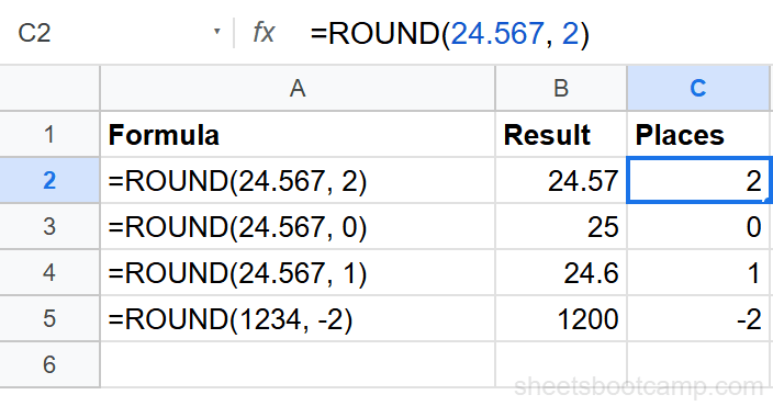
=ROUND(24.567, 2) | 24.57 | Rounds to 2 decimal places |
=ROUND(24.567, 0) | 25 | Rounds to nearest whole number |
=ROUND(24.567, 1) | 24.6 | Rounds to 1 decimal place |
=ROUND(1234, -2) | 1200 | Rounds to nearest hundred |
ROUNDUP: Always Round Away from Zero
ROUNDUP always rounds away from zero, regardless of the next digit. This is useful when you need to round up for pricing, billing, or inventory calculations.
=ROUNDUP(value, [places])| Formula | Result | Explanation |
|---|---|---|
=ROUNDUP(24.321, 2) | 24.33 | Rounds up to 2 decimal places |
=ROUNDUP(24.001, 0) | 25 | Rounds up to next whole number |
=ROUNDUP(-3.2, 0) | -4 | Rounds away from zero (more negative) |
ROUNDUP rounds away from zero in both directions. Positive numbers get larger, negative numbers get more negative. =ROUNDUP(-3.2, 0) returns -4, not -3.
ROUNDDOWN: Always Round Toward Zero
ROUNDDOWN always rounds toward zero, discarding the extra digits. This is how truncation works. Useful when you need to drop decimals without rounding up.
=ROUNDDOWN(value, [places])| Formula | Result | Explanation |
|---|---|---|
=ROUNDDOWN(24.999, 2) | 24.99 | Drops digits beyond 2 places |
=ROUNDDOWN(24.999, 0) | 24 | Drops all decimal digits |
=ROUNDDOWN(-3.9, 0) | -3 | Rounds toward zero (less negative) |
MROUND: Round to a Multiple
MROUND rounds a number to the nearest multiple of another number. Use it when you need values to land on a specific interval like 5, 10, 25, or 0.25.
=MROUND(value, factor)| Argument | Description | Required |
|---|---|---|
| value | The number to round | Yes |
| factor | The multiple to round to | Yes |
| Formula | Result | Explanation |
|---|---|---|
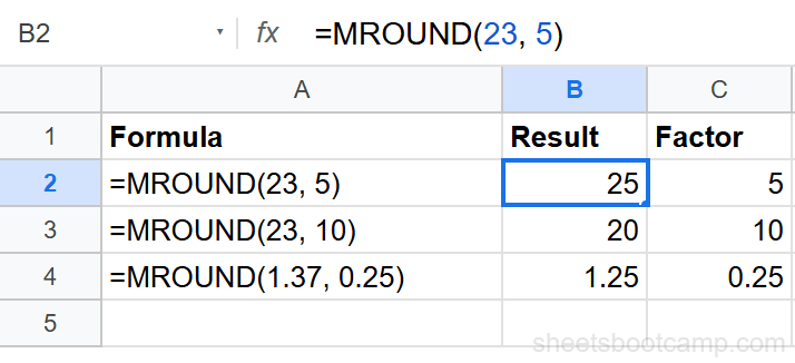
=MROUND(23, 5) | 25 | Rounds to nearest 5 |
=MROUND(23, 10) | 20 | Rounds to nearest 10 |
=MROUND(1.37, 0.25) | 1.25 | Rounds to nearest quarter |
Both arguments in MROUND must have the same sign. =MROUND(23, -5) returns a #NUM! error because the value is positive and the factor is negative.
How to Round Numbers: Step-by-Step
Enter the ROUND formula
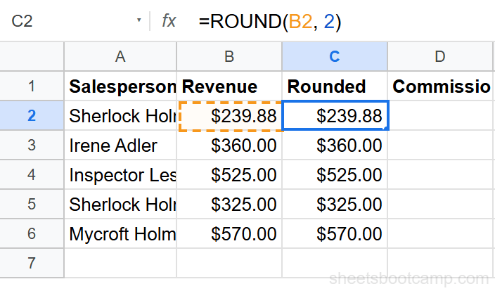
Select the cell where you want the rounded result. Type =ROUND( followed by the cell reference or number, a comma, and the number of decimal places.
For example, enter =ROUND(B2, 2) in cell C2 to round the value in B2 to two decimal places.
Choose the right function
Decide which rounding behavior you need:
- Standard rounding (5+ rounds up, 4 and below rounds down): use
ROUND - Always round up (for pricing, billing, material estimates): use
ROUNDUP - Always round down (for truncation, conservative estimates): use
ROUNDDOWN - Round to a specific increment (nearest 5, 10, quarter-hour): use
MROUND
Verify the result
Check the output against the original number. If you rounded $239.88 to 0 places with ROUND, expect $240. With ROUNDDOWN, expect $239. With ROUNDUP, expect $240.
Use negative values for the places argument to round large numbers. =ROUND(15678, -3) returns 16000. This is useful for rounding revenue or population figures to the nearest thousand.
Practical Examples
Example 1: Round Commission to Two Decimal Places
You have a commission rate of 10% applied to revenue values. The raw calculation produces long decimals.
=ROUND(F2 * 0.10, 2)If F2 contains $239.88, this returns $23.99. Without ROUND, you’d see $23.988.
Example 2: Round Hours Up for Billing
A freelancer bills in whole-hour increments. Any partial hour rounds up to the next full hour.
=ROUNDUP(A2, 0)If A2 contains 3.25 (three and a quarter hours), this returns 4. The client is billed for 4 hours.
Example 3: Round Prices to Nearest Quarter
A pricing model requires all prices to end in .00, .25, .50, or .75.
=MROUND(A2, 0.25)If A2 contains $24.37, this returns $24.25. If A2 contains $24.88, this returns $25.00.
ROUND vs Number Formatting
ROUND and number formatting look similar but work differently. This distinction matters when other formulas reference the rounded cell.
| ROUND Function | Number Formatting | |
|---|---|---|
| Changes the stored value | Yes | No |
| Affects downstream formulas | Yes | No |
| How to apply | Formula: =ROUND(A1, 2) | Format > Number > Custom |
| Reversible | Delete the formula | Change the format back |
If you format a cell to show 2 decimal places, the display shows 24.57 but the cell still stores 24.567. Any SUM or AVERAGE referencing that cell uses 24.567. If you wrap it in ROUND, the stored value becomes 24.57 and all downstream formulas use 24.57.
For number formatting details, see the full guide.
Common Errors and How to Fix Them
#NUM! Error in MROUND
The value and factor must have the same sign. =MROUND(-10, 3) returns #NUM! because -10 is negative and 3 is positive. Fix it by matching signs: =MROUND(-10, -3) returns -9.
#VALUE! Error
The arguments are not numbers. Check for text in the referenced cells. Use =ISNUMBER(A2) to verify. If the cell contains a number formatted as text, multiply by 1 or use =VALUE(A2) to convert it.
Unexpected Rounding with Floating Point
Google Sheets uses floating-point arithmetic. Occasionally, =0.1 + 0.2 returns 0.30000000000000004 instead of 0.3. Wrap the calculation in ROUND to clean up the result: =ROUND(0.1 + 0.2, 1) returns 0.3.
Tips and Best Practices
- Round at the end, not in the middle. If a formula chains multiple calculations, apply ROUND to the final result. Rounding intermediate values introduces cumulative rounding errors.
- Use ROUND(value, 0) for whole numbers. This is cleaner than ROUNDDOWN or INT when you want standard rounding to the nearest integer.
- Use MROUND for time rounding.
=MROUND(A1, TIME(0,15,0))rounds a time value to the nearest 15-minute increment. Useful for timesheet calculations. - Pair with IF statements for conditional rounding.
=IF(A2>100, ROUND(A2, 0), ROUND(A2, 2))rounds large values to whole numbers and small values to two decimal places. - Check currency columns. Revenue and price columns often need
=ROUND(value, 2)to avoid long decimal strings from multiplication.
Related Google Sheets Tutorials
- IF Function in Google Sheets — Combine IF with ROUND for conditional rounding based on value thresholds
- Custom Number Formats in Google Sheets — Control how numbers display without changing the stored value
- AVERAGE, AVERAGEIF, and AVERAGEIFS — Round average results to a clean number of decimal places
- COUNT, COUNTA, COUNTBLANK — Count values in ranges before applying rounding to totals
FAQ
What is the difference between ROUND and ROUNDUP in Google Sheets?
ROUND follows standard rounding rules and rounds to the nearest value. ROUNDUP always rounds away from zero regardless of the digit. ROUND(2.34, 1) returns 2.3, while ROUNDUP(2.34, 1) returns 2.4.
How do I round to the nearest dollar in Google Sheets?
Use =ROUND(A1, 0) to round to the nearest whole number. This rounds 24.49 to 24 and 24.50 to 25. Use ROUNDUP(A1, 0) if you always want to round up to the next dollar.
How do I round to the nearest 5 or 10 in Google Sheets?
Use the MROUND function. =MROUND(A1, 5) rounds to the nearest 5, and =MROUND(A1, 10) rounds to the nearest 10. For example, MROUND(23, 5) returns 25 and MROUND(23, 10) returns 20.
What does a negative places value do in ROUND?
A negative places value rounds to the left of the decimal point. ROUND(1234, -1) returns 1230 (nearest ten), ROUND(1234, -2) returns 1200 (nearest hundred), and ROUND(1234, -3) returns 1000 (nearest thousand).
Does ROUND change the actual value or just the display?
ROUND changes the actual value stored in the cell. This is different from number formatting (Format > Number), which only changes how the value displays. If you ROUND 2.567 to 2.57, any formula referencing that cell uses 2.57.
Can I round time values in Google Sheets?
Yes. Use MROUND to round times to the nearest interval. =MROUND(A1, TIME(0,15,0)) rounds a time to the nearest 15 minutes. =MROUND(A1, TIME(0,30,0)) rounds to the nearest half hour.