TRANSPOSE in Google Sheets: Flip Rows and Columns
Learn how to use the TRANSPOSE function in Google Sheets to flip rows into columns and columns into rows. Covers the formula, paste special, and tips.
Sheets Bootcamp
March 13, 2026 · Updated June 22, 2026
TRANSPOSE in Google Sheets flips your data so rows become columns and columns become rows. The TRANSPOSE function creates a live link to the source data, meaning the transposed output updates automatically when the original values change.
This guide covers the TRANSPOSE function syntax, the Paste Special shortcut for static transposing, and how to fix common errors when your output range runs into existing data.
In This Guide
- What Is TRANSPOSE?
- Syntax and Parameters
- How to Use TRANSPOSE: Step-by-Step
- TRANSPOSE Examples
- Common Errors and How to Fix Them
- Tips and Best Practices
- Related Google Sheets Tutorials
- FAQ
What Is TRANSPOSE?
TRANSPOSE rotates the orientation of a range. A horizontal row of data becomes a vertical column, and a vertical column becomes a horizontal row. A range that’s 3 rows by 5 columns becomes 5 rows by 3 columns.
This is useful when data arrives in a layout that doesn’t work for your analysis. Monthly totals listed across columns might need to run down a column for charting. Survey responses in a single row might need to stack vertically for review.
Syntax and Parameters
=TRANSPOSE(range_or_array)| Parameter | Description | Required |
|---|---|---|
| range_or_array | The range or array to transpose. Rows become columns and columns become rows | Yes |
TRANSPOSE spills its output into adjacent cells. If your source data is 4 rows by 6 columns, the output needs 6 rows by 4 columns of empty space. Any data in those cells causes a #REF! error.
How to Use TRANSPOSE: Step-by-Step
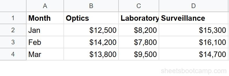
We’ll transpose a summary table from a horizontal layout to a vertical one.
Select your source data
The source data is in cells A1:D4 — four columns (Month, Optics, Laboratory, Surveillance) and four rows (header plus three months of data).
Enter the TRANSPOSE formula
Click cell F1 (or any cell with enough empty space). Enter the formula:
=TRANSPOSE(A1:D4)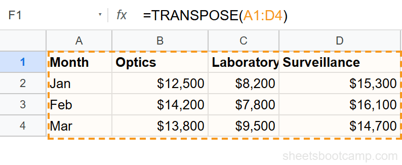
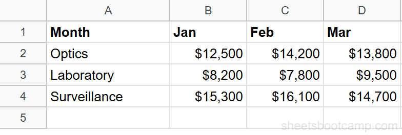
Review the transposed output
The data now flows in the opposite direction. What were column headers (Month, Optics, Laboratory, Surveillance) now run down column F. Each month’s values fill a column to the right.
For a one-time paste without formulas, copy your range, right-click the destination, and select Paste Special > Paste transposed. This creates a static copy with formatting intact.
TRANSPOSE Examples
Transpose a Single Row to a Column
Turn a horizontal header row into a vertical list:
=TRANSPOSE(A1:G1)A row of 7 values in A1:G1 becomes a column of 7 values. This is useful for creating label lists from headers.
Transpose a Column to a Row
Stack monthly totals stored in a column into a single row for a chart:
=TRANSPOSE(B2:B13)Twelve values in B2:B13 become a single row of 12 values. This works well when you need horizontal data for sparklines or dashboard layouts.
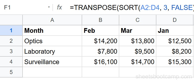
Combine TRANSPOSE with SORT
Sort data by a column, then transpose the sorted result:
=TRANSPOSE(SORT(A2:D7, 3, FALSE))This sorts the data by column 3 in descending order first, then transposes the sorted output. Each original row becomes a column in the final result.
Common Errors and How to Fix Them
#REF! Error
The output area contains existing data. TRANSPOSE needs the destination cells to be empty. If your source is 4 rows by 3 columns, clear at least 3 rows by 4 columns at the destination.
#VALUE! Error
The argument is a single cell, not a range. TRANSPOSE needs at least a 1-by-2 or 2-by-1 range to flip. Passing a single cell like =TRANSPOSE(A1) returns a #VALUE! error.
Partial Data Showing
The TRANSPOSE formula isn’t expanding into all cells. This can happen if merged cells block the spill area. Unmerge any cells in the output range and try again.
If you need to transpose data but keep cell formatting (colors, borders, number formats), use Paste Special > Paste transposed instead of the formula. The function only carries values.
Tips and Best Practices
-
Use TRANSPOSE for dashboard layouts. Source data often arrives in a table format that doesn’t fit a dashboard design. TRANSPOSE lets you reshape it without restructuring the original.
-
Pair with ARRAYFORMULA for calculated transpositions. Wrap calculations inside TRANSPOSE:
=TRANSPOSE(ARRAYFORMULA(B2:B7*1.1))transposes a column of values after applying a 10% increase. -
Clear the destination area first. TRANSPOSE spills into adjacent cells. Any existing values cause #REF! errors. Use a dedicated output area or an empty sheet tab.
-
Remember: the function version is live. Changes to the source data update the transposed output. If you want a frozen snapshot, use Paste Special instead.
-
Check dimensions before transposing large ranges. A range that’s 100 rows by 3 columns becomes 3 rows by 100 columns. Make sure your sheet has enough columns to accommodate the result.
Related Google Sheets Tutorials
- ARRAYFORMULA Complete Guide - Apply formulas to entire columns and combine with TRANSPOSE for array operations
- QUERY Function: The Complete Guide - Reshape and aggregate data using SQL-like syntax
- Paste Special in Google Sheets - Transpose data with formatting using Paste Special > Paste transposed
- SORT Function in Google Sheets - Sort data before transposing for organized output
FAQ
How do I transpose data in Google Sheets?
Use the TRANSPOSE function: =TRANSPOSE(A1:D10). This flips your data so rows become columns and columns become rows. The result is a live formula that updates when the source changes. For a static copy, use Paste Special > Transposed instead.
How do I flip rows and columns without a formula?
Copy your data range, right-click the destination cell, select Paste Special > Paste transposed. This creates a static copy with rows and columns swapped. Unlike the TRANSPOSE function, this paste doesn’t update when the source changes.
Why does TRANSPOSE return a #REF! error?
The transposed output doesn’t have enough room to spill. If your source is 3 rows by 5 columns, the output needs 5 rows by 3 columns of empty space. Clear the cells in the destination area or move the formula.
Can I transpose and keep formatting?
The TRANSPOSE function only carries values and formulas, not formatting. To keep formatting, use Paste Special > Paste transposed, which preserves cell colors, borders, and number formats from the original range.
Can I use TRANSPOSE with other functions?
Yes. TRANSPOSE works inside other functions. For example, =QUERY(TRANSPOSE(A1:D4), "SELECT *") transposes data before querying it. You can also nest TRANSPOSE inside SORT, FILTER, or ARRAYFORMULA.
What is the difference between TRANSPOSE function and Paste Transposed?
The TRANSPOSE function creates a live link to the source data that updates automatically. Paste Transposed creates a static one-time copy. Use the function when the source data changes. Use paste when you need a fixed snapshot.