UNIQUE Function in Google Sheets (Formula Guide)
Learn how to use the UNIQUE function in Google Sheets to extract distinct values from a column or range. Covers syntax, examples, and combining with SORT.
Sheets Bootcamp
March 13, 2026 · Updated June 15, 2026
The UNIQUE function in Google Sheets extracts distinct values from a column or range and returns them as a list without duplicates. It outputs the results to a new location and leaves the original data untouched.
This guide covers UNIQUE syntax, extracting unique values from single and multiple columns, combining UNIQUE with SORT and FILTER, and handling common issues.
In This Guide
- What Is the UNIQUE Function?
- Syntax and Parameters
- How to Use UNIQUE: Step-by-Step
- UNIQUE Examples
- Common Errors and How to Fix Them
- Tips and Best Practices
- Related Google Sheets Tutorials
- FAQ
What Is the UNIQUE Function?
UNIQUE scans a range and returns each distinct value once. If a column contains “Baker Street” five times, UNIQUE returns it once. The output updates automatically when the source data changes.
Use UNIQUE when you need a clean list of categories, names, or labels from a column that contains repeated entries — like building a dropdown list from existing data, or creating a summary that lists each region or product once.
Syntax and Parameters
=UNIQUE(range)| Parameter | Description | Required |
|---|---|---|
| range | The column or range to extract unique values from | Yes |
UNIQUE in Google Sheets takes only one argument. This is different from Excel’s UNIQUE, which has additional parameters for exactly_once and by_column. In Google Sheets, UNIQUE always returns all distinct values.
How to Use UNIQUE: Step-by-Step
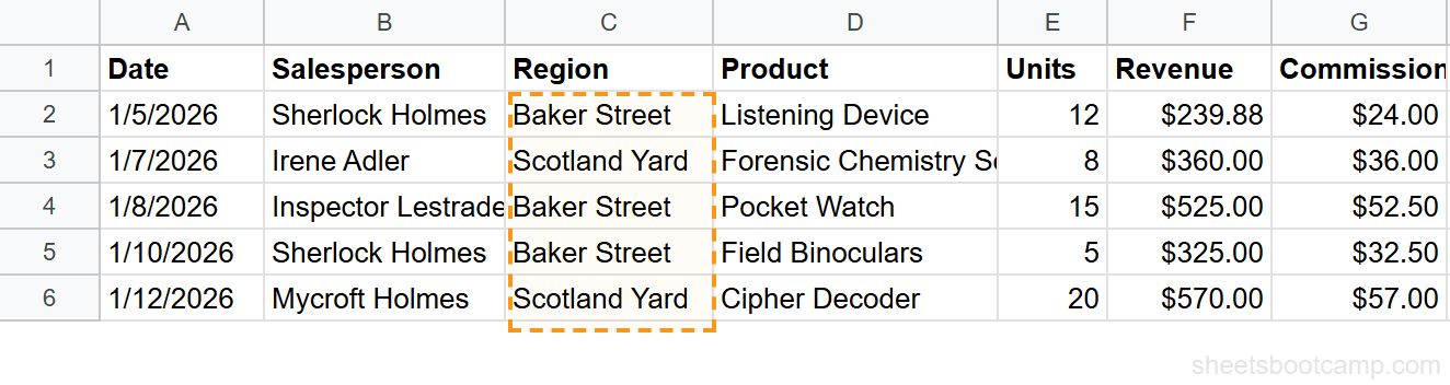
We’ll extract a unique list of regions from a sales dataset.
Identify the column with duplicates
The sales data has 18 rows with a Region column (C) containing repeated values: Baker Street, Scotland Yard, and Whitehall appear multiple times.
Enter the UNIQUE formula
Click cell I2 and enter the formula:
=UNIQUE(C2:C19)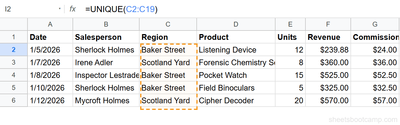
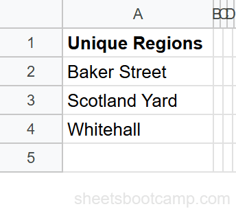
Review the unique list
The formula returns three values: Baker Street, Scotland Yard, and Whitehall — one instance of each region in the order they first appear in the data.
UNIQUE is case-sensitive. “baker street” and “Baker Street” are treated as different values. Clean your data with TRIM and PROPER before applying UNIQUE if casing is inconsistent.
UNIQUE Examples
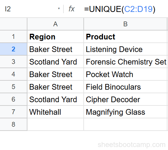
Unique Values from Multiple Columns
Extract unique rows based on the combination of Region and Product:
=UNIQUE(C2:D19)This returns every distinct Region-Product pair. Two rows with the same region but different products are treated as separate entries.
Sorted Unique List
Extract unique salesperson names and sort them alphabetically:
=SORT(UNIQUE(B2:B19))UNIQUE pulls the distinct names, and SORT arranges them A-Z. This is useful for building dropdown lists or summary headers.
Unique Values Excluding Blanks
If your data has empty cells, UNIQUE returns a blank row. Filter those out:
=UNIQUE(FILTER(C2:C100, C2:C100<>""))FILTER removes blank cells first, then UNIQUE extracts the distinct values from the filtered result.
Count of Unique Values
Get the number of unique entries in a column:
=COUNTA(UNIQUE(C2:C19))UNIQUE returns the list, and COUNTA counts how many non-empty values are in it. For this dataset, it returns 3 (the three regions).
Common Errors and How to Fix Them
#REF! Error
The output doesn’t have enough room to spill. UNIQUE needs empty cells below the formula to display all unique values. Clear the cells below the formula, or move it to an area with enough space.
Unexpected Duplicates in Output
UNIQUE is case-sensitive and space-sensitive. “Whitehall” and “Whitehall ” (with a trailing space) are different values. Use =UNIQUE(TRIM(C2:C19)) to strip extra spaces, or =UNIQUE(LOWER(C2:C19)) to normalize casing.
UNIQUE with TRIM or LOWER nested inside works in Google Sheets because these functions accept array arguments. This is a Google Sheets feature — Excel handles this differently.
Blank Row in Output
Your source range extends beyond the actual data and includes empty cells. UNIQUE treats one blank as a unique value. Either tighten the range to match your data, or wrap in FILTER to exclude blanks.
Tips and Best Practices
-
Build dynamic dropdown lists. Use UNIQUE output as the source for a data validation dropdown. The dropdown automatically updates when new values appear in the source data.
-
Combine with COUNTA for quick counts. =COUNTA(UNIQUE(range)) tells you how many distinct values exist without needing a pivot table.
-
Pair with SORT for clean lists. UNIQUE preserves the order values first appear. Wrap in SORT if you need alphabetical or numerical order.
-
Use UNIQUE on multiple columns for deduplication. =UNIQUE(A2:D100) returns rows where the full combination of columns is unique — a formula-based alternative to Remove Duplicates.
-
Watch for case mismatches. UNIQUE treats “North” and “north” as different. Standardize casing in the source data or wrap in UPPER/LOWER inside the UNIQUE formula.
Related Google Sheets Tutorials
- How to Remove Duplicates in Google Sheets - Five methods including UNIQUE, menu option, and COUNTIF approach
- SORT Function in Google Sheets - Sort data with formulas and combine with UNIQUE for sorted unique lists
- FILTER Function Complete Guide - Filter rows by condition and pair with UNIQUE for targeted deduplication
- Google Sheets QUERY Function - Use SELECT DISTINCT in QUERY as an alternative to UNIQUE
FAQ
How do I get unique values in Google Sheets?
Use =UNIQUE(range) where range is the column or area containing duplicates. The function returns each distinct value once, in the order it first appears. For example, =UNIQUE(A2:A100) returns a deduplicated list from column A.
What is the difference between UNIQUE and Remove Duplicates?
UNIQUE is a formula that outputs deduplicated values to a new location without touching the original data. Remove Duplicates (Data menu) permanently deletes duplicate rows from the source data. Use UNIQUE when you want to keep the original intact.
Can UNIQUE work on multiple columns?
Yes. =UNIQUE(A2:C10) returns rows where the combination of all columns is unique. Two rows with the same value in column A but different values in column B are treated as distinct.
How do I sort unique values in Google Sheets?
Wrap UNIQUE inside SORT: =SORT(UNIQUE(A2:A100)). This extracts distinct values and sorts them alphabetically. Add FALSE as the third argument to sort Z-A.
Why does UNIQUE return blank rows?
Your source range includes empty cells. UNIQUE treats blanks as a unique value and returns one blank row. Either shrink your range to exclude blanks, or wrap in FILTER: =UNIQUE(FILTER(A2:A100, A2:A100<>"")).
Does UNIQUE preserve the original order?
Yes. UNIQUE returns values in the order they first appear in the source range. The first occurrence of each value determines its position in the output.