VLOOKUP Approximate vs Exact Match in Google Sheets
Learn the difference between VLOOKUP approximate match (TRUE) and exact match (FALSE) in Google Sheets. When to use each with step-by-step examples.
Sheets Bootcamp
March 14, 2026 · Updated April 24, 2026
VLOOKUP in Google Sheets has a fourth argument that controls how it searches: exact match (FALSE) or approximate match (TRUE). Most tutorials only cover exact match, but approximate match is the right tool for grading scales, tax brackets, commission tiers, and any lookup where values fall between thresholds.
This guide explains how both modes work, when to use each, and why leaving the argument blank is dangerous.
In This Guide
- Exact Match vs Approximate Match
- How Exact Match Works (FALSE)
- How Approximate Match Works (TRUE)
- Step-by-Step: Grade Calculator with Approximate Match
- The Default Trap: Omitting the Fourth Argument
- Common Errors and How to Fix Them
- Tips and Best Practices
- Related Google Sheets Tutorials
- Frequently Asked Questions
Exact Match vs Approximate Match
The fourth argument in VLOOKUP (is_sorted) controls the search behavior:
| Value | Mode | How it searches | Use case |
|---|---|---|---|
FALSE | Exact match | Finds the search key exactly as entered | Product IDs, employee names, specific codes |
TRUE | Approximate match | Finds the largest value ≤ the search key | Grade scales, tax brackets, commission tiers |
=VLOOKUP(search_key, range, index, TRUE or FALSE)If you omit the fourth argument, VLOOKUP defaults to TRUE (approximate match). On unsorted data, this returns wrong results without any error message. Always specify FALSE unless you need approximate matching on sorted data.
How Exact Match Works (FALSE)
Exact match is the more common mode. VLOOKUP scans the first column for a value that matches your search key character for character.
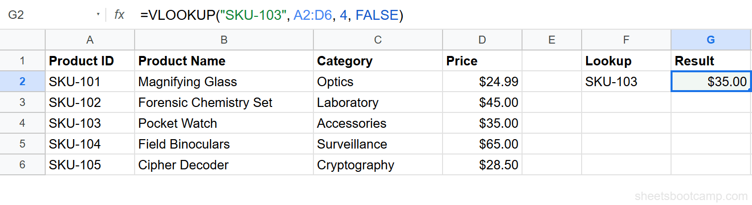
=VLOOKUP("SKU-103", A2:D6, 4, FALSE)This searches column A for the exact text “SKU-103” and returns $35.00 from column D.
If the value does not exist, VLOOKUP returns #N/A. There is no ambiguity: it either finds the value or it does not.
When to use exact match:
- Looking up product IDs, employee IDs, or codes
- Matching names or text values
- Any time the search key must exist exactly in the data
How Approximate Match Works (TRUE)
Approximate match finds the largest value in the first column that is less than or equal to your search key. The first column must be sorted in ascending order.
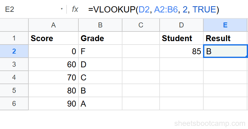
Consider this grading scale:
| Score Threshold | Grade |
|---|---|
| 0 | F |
| 60 | D |
| 70 | C |
| 80 | B |
| 90 | A |
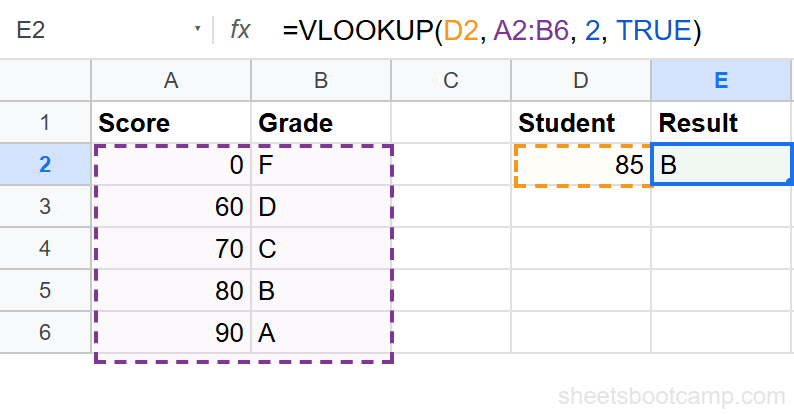
=VLOOKUP(85, A2:B6, 2, TRUE)The score 85 does not appear in column A. VLOOKUP finds the largest threshold ≤ 85, which is 80, and returns “B.”
Here is how VLOOKUP evaluates each row:
| Threshold | Comparison | Result |
|---|---|---|
| 0 | 85 ≥ 0 | Possible match |
| 60 | 85 ≥ 60 | Better match (closer) |
| 70 | 85 ≥ 70 | Better match |
| 80 | 85 ≥ 80 | Best match (largest ≤ 85) |
| 90 | 85 < 90 | Too high, skip |
VLOOKUP returns the row for threshold 80 because it is the largest value that does not exceed 85.
Step-by-Step: Grade Calculator with Approximate Match
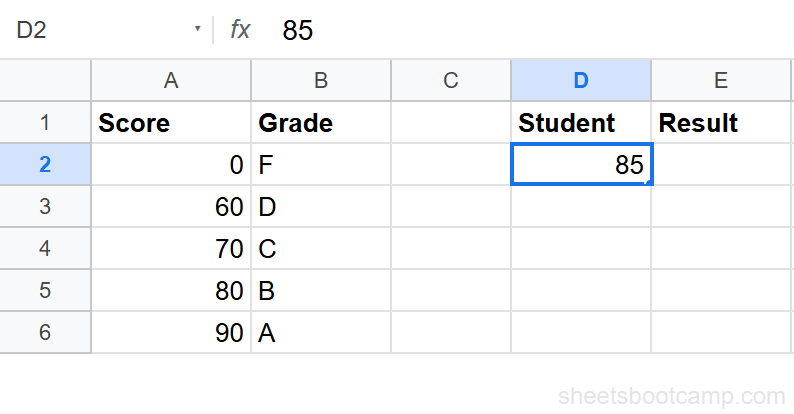
Set up a grading scale table sorted in ascending order
Create the grading scale in columns A and B. The score thresholds must be sorted from lowest to highest. Enter a student score (85) in cell D2.
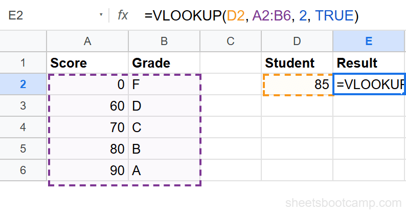
Write the VLOOKUP formula with TRUE for approximate match
Enter the following formula in cell E2:
=VLOOKUP(D2, A2:B6, 2, TRUE)D2 is the student score. A2:B6 is the grading scale. 2 returns the Grade column. TRUE enables approximate matching.
Review how approximate match selects the correct row
The formula returns “B” because 85 falls between the 80 threshold (B) and 90 threshold (A). VLOOKUP picks 80 as the match.
Change D2 to 92 and the result updates to “A.” Change it to 55 and the result is “F.”
The thresholds must be sorted in ascending order. If you rearrange the rows (put 90 before 60, for example), VLOOKUP returns wrong results silently.
The Default Trap: Omitting the Fourth Argument
VLOOKUP defaults to TRUE when you leave out the fourth argument:
=VLOOKUP("SKU-103", A2:D6, 4)This formula uses approximate match even though you probably want exact match. If the data happens to be sorted alphabetically, it may return a result that looks correct. If the data is not sorted, it returns the wrong value with no warning.
This is the most common source of VLOOKUP bugs. Two formulas that look nearly identical produce different results:
| Formula | Mode | Result |
|---|---|---|
=VLOOKUP("SKU-103", A2:D6, 4, FALSE) | Exact | $35.00 (correct) |
=VLOOKUP("SKU-103", A2:D6, 4) | Approximate (default) | May return wrong value |
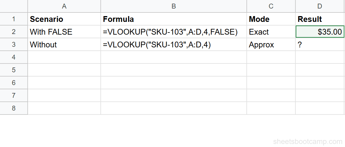
Always include the fourth argument. Typing , FALSE takes two seconds. Debugging a wrong result caused by the default TRUE on unsorted data takes much longer.
Common Errors and How to Fix Them
Wrong Result (No Error Message)
This is the most dangerous outcome. VLOOKUP returns a value, but it is the wrong value. It happens when:
- You use
TRUEon unsorted data - You omit the fourth argument (defaults to
TRUE)
Fix: Sort the first column in ascending order, or switch to FALSE for exact match.
#N/A Error with Approximate Match
With TRUE, VLOOKUP returns #N/A only when the search key is smaller than every value in the first column. For example, looking up a score of -5 in a grading scale that starts at 0.
Fix: Add a row with the lowest possible value (0 in a grading scale) to catch all inputs.
#N/A Error with Exact Match
The search key does not exist in the first column. Check for typos, extra spaces, or mismatched data types (text vs number).
Fix: Use TRIM to clean data, or wrap in IFERROR to handle missing values: =IFERROR(VLOOKUP(D2, A2:B6, 2, FALSE), "Not found").
Tips and Best Practices
-
Default to
FALSEfor everyday lookups. Exact match is the right choice for product IDs, names, and codes. Only useTRUEwhen your data represents ranges or thresholds. -
Sort ascending before using approximate match. VLOOKUP with
TRUErequires the first column sorted from smallest to largest (numbers) or A to Z (text). There is no error message if this requirement is not met. -
Use approximate match for grading, tiering, and bracketing. Tax brackets, shipping rates, commission schedules, and performance ratings are natural fits.
-
Test edge cases. For a grading scale from 0 to 90, test values like 0 (lowest threshold), 59 (just below next tier), 60 (on a threshold), and 100 (above highest threshold).
-
Consider INDEX MATCH for complex scenarios. INDEX MATCH does not have a built-in approximate match mode, but combining it with MAX or MATCH gives you the same result with more flexibility.
Related Google Sheets Tutorials
- VLOOKUP in Google Sheets - Complete guide to VLOOKUP syntax and features
- VLOOKUP for Beginners - Step-by-step first VLOOKUP tutorial
- Fix VLOOKUP Errors - Troubleshoot #N/A, #REF!, and #VALUE! errors
- VLOOKUP with Wildcards - Partial text matching with asterisk and question mark
- INDEX MATCH in Google Sheets - A flexible alternative to VLOOKUP
Frequently Asked Questions
What is the difference between TRUE and FALSE in VLOOKUP?
FALSE finds an exact match for your search key. TRUE finds the largest value less than or equal to your search key (approximate match). FALSE is the safer default. TRUE requires sorted data and returns wrong results silently if the first column is not sorted in ascending order.
When should I use approximate match in VLOOKUP?
Use approximate match (TRUE) for range-based lookups like grading scales, tax brackets, commission tiers, or shipping rates where values fall between thresholds rather than matching exactly.
What happens if I omit the last argument in VLOOKUP?
VLOOKUP defaults to TRUE (approximate match). This catches many beginners off guard because the formula appears to work but may return incorrect results on unsorted data. Always specify FALSE unless you intentionally need an approximate match.
Does approximate match VLOOKUP require sorted data?
Yes. The first column of your range must be sorted in ascending order (A to Z or smallest to largest). If the data is not sorted, VLOOKUP with TRUE returns unpredictable results without any error message.
Can approximate match VLOOKUP return the wrong result?
Yes. If the first column is not sorted in ascending order, approximate match returns incorrect values without triggering an error. This makes it one of the most common sources of silent spreadsheet mistakes.