How to VLOOKUP Dates in Google Sheets
Learn how to VLOOKUP dates in Google Sheets. Fix date format mismatches, use DATEVALUE for text dates, and look up date ranges with step-by-step examples.
Sheets Bootcamp
March 15, 2026 · Updated August 24, 2026
VLOOKUP dates in Google Sheets works the same as any other VLOOKUP lookup, but dates have a hidden layer that causes problems. Dates in Google Sheets are numbers wearing a disguise. What you see as “1/5/2026” is actually the serial number 46023 under the hood.
When VLOOKUP compares dates, it compares those serial numbers. If the lookup value and the data column store dates differently (one as a real date, the other as text), VLOOKUP returns #N/A even when the dates look identical on screen. This guide covers how to match dates reliably, fix text-vs-date mismatches, and use approximate match for date range lookups.
In This Guide
- Why Dates Cause VLOOKUP Problems
- How to VLOOKUP a Date: Step-by-Step
- VLOOKUP Date Examples
- Common Errors and How to Fix Them
- Tips and Best Practices
- Related Google Sheets Tutorials
- Frequently Asked Questions
Why Dates Cause VLOOKUP Problems
Google Sheets stores every date as a serial number. January 1, 1900 is serial number 1. Each day after that adds 1 to the count. January 5, 2026 is 46023.
When you type “1/5/2026” into a cell, Sheets usually recognizes it as a date and stores it as 46023. But sometimes it does not. Data imported from CSVs, pasted from websites, or pulled with IMPORTRANGE can arrive as text that looks like a date but is not.
VLOOKUP compares the underlying values, not the formatting. A real date (46023) and the text “1/5/2026” are completely different data types. VLOOKUP treats them as non-matching, and you get #N/A.
Here is how to tell the difference:
| What you see | What VLOOKUP sees | =ISNUMBER() result |
|---|---|---|
| 1/5/2026 (real date) | 46023 | TRUE |
| 1/5/2026 (text) | “1/5/2026” | FALSE |
Use =ISNUMBER(A2) to check whether a cell contains a real date or text. If it returns FALSE, the cell holds text. VLOOKUP will not match a real date against a text date, even if they look identical.
How to VLOOKUP a Date: Step-by-Step
We’ll use a sales records table with 18 rows of data. Column A has dates from 1/5/2026 to 2/7/2026. The goal: look up a specific date and return the revenue from that sale.
Set up the sales data with dates in column A
Your data has dates in column A, salesperson in column B, and revenue in column F. The dates are real date values (not text).
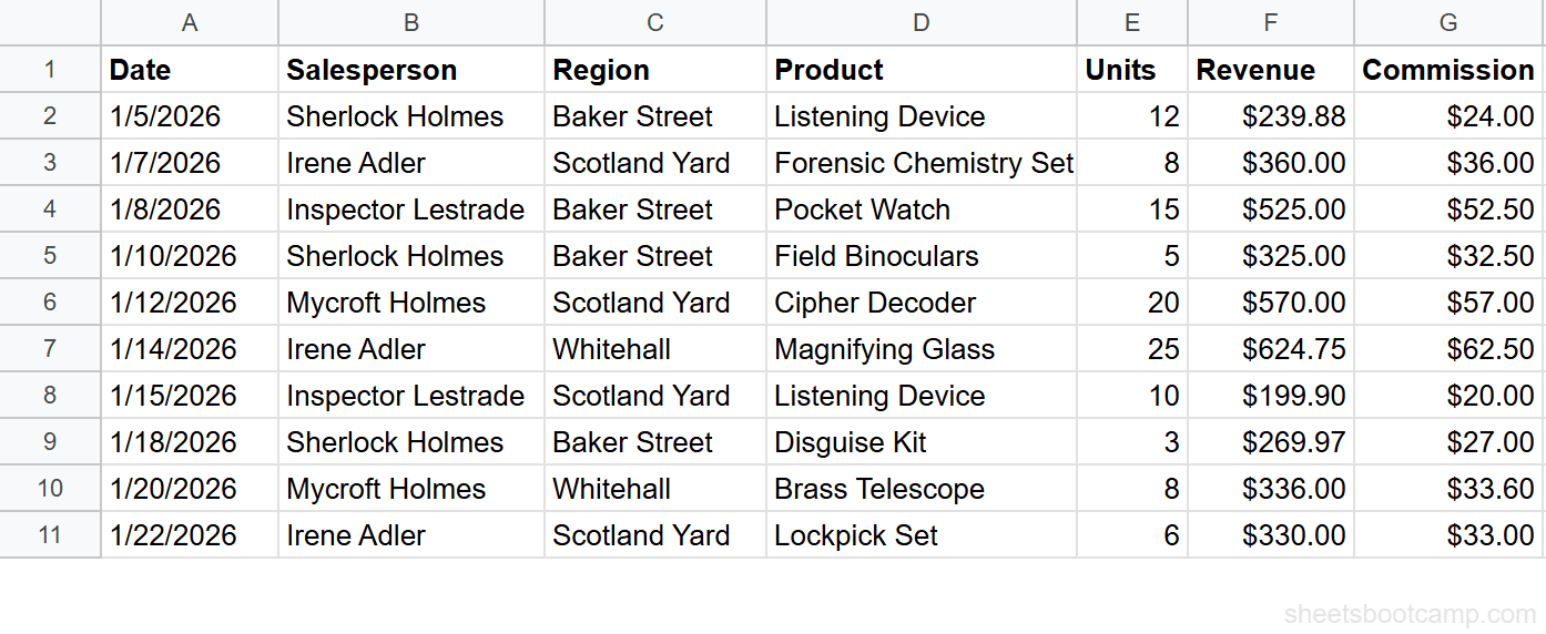
Select column A, then check Format > Number. If it says “Date,” the values are real dates. If it says “Plain text” or “Automatic,” select the cells and apply Format > Number > Date to convert them.
Write the VLOOKUP formula with a DATE function as the lookup value
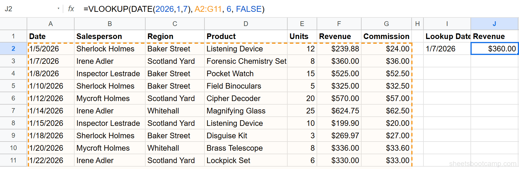
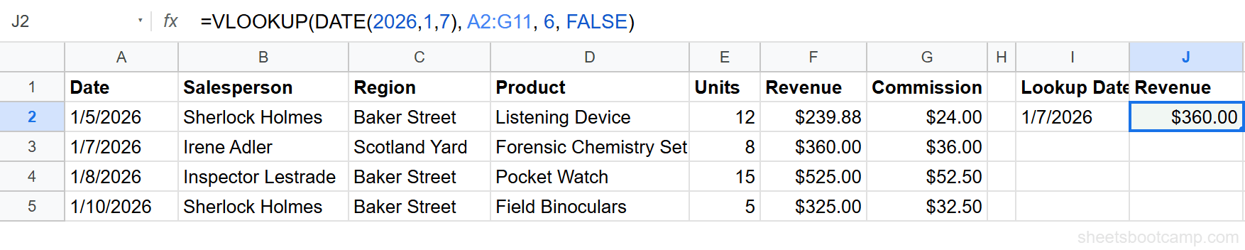
Enter the following formula in an empty cell:
=VLOOKUP(DATE(2026,1,7), A2:G19, 6, FALSE)The DATE function creates the serial number for January 7, 2026. Using DATE(2026,1,7) instead of typing “1/7/2026” guarantees you are passing a real date value, not text.
DATE(2026,1,7)is the lookup value (January 7, 2026)A2:G19is the data range (dates in column A)6returns the sixth column (Revenue)FALSErequires an exact match
Always use the DATE function or a cell reference for your lookup value. Typing a date directly as text like "1/10/2026" can create a text string instead of a real date, which causes #N/A errors.
Verify the result and troubleshoot mismatches
The formula returns $360.00. That is the revenue from Irene Adler’s sale of a Forensic Chemistry Set on January 7, 2026.
If you get #N/A, check both the lookup value and the date column with =ISNUMBER(). Both must return TRUE for the match to work.
VLOOKUP Date Examples
Example 1: Look Up a Date from a Cell Reference
Instead of hardcoding the date in the formula, reference a cell where the user enters a date. Place “1/7/2026” in cell I2, then use:
=VLOOKUP(I2, A2:G19, 2, FALSE)This returns “Irene Adler,” the salesperson for that date. Make sure I2 contains a real date value, not text.
Example 2: Fix Text Dates with DATEVALUE
When dates arrive as text (common with CSV imports), VLOOKUP cannot match them against real dates. DATEVALUE converts the text to a real date serial number.
If cell I2 contains the text “1/7/2026” (not a real date), this standard VLOOKUP fails:
=VLOOKUP(I2, A2:G19, 6, FALSE)Wrap the lookup value in DATEVALUE to fix it:
=VLOOKUP(DATEVALUE(I2), A2:G19, 6, FALSE)This returns $360.00, the revenue from the January 7, 2026 sale. DATEVALUE converts the text “1/7/2026” into the serial number 46025, which matches the real date in column A.
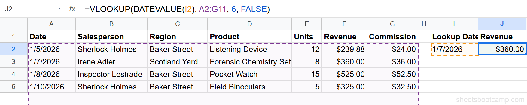
If the dates in your data column are also text, convert them first. You can add a helper column with =DATEVALUE(A2) and point VLOOKUP at that column instead.
Example 3: Approximate Match for Date Ranges
Approximate match (TRUE) finds the closest date on or before your lookup date. This is useful when you need to find which record was most recent as of a given date.
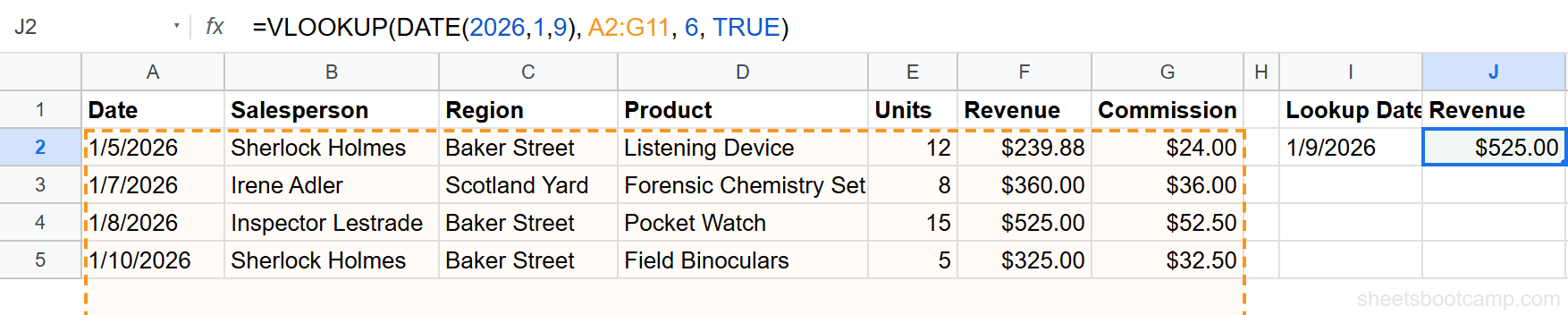
The sales data has entries on 1/5, 1/7, 1/8, 1/10, 1/12, and so on. What if you want the last sale on or before January 9?
=VLOOKUP(DATE(2026,1,9), A2:G19, 6, TRUE)January 9 does not appear in the data. VLOOKUP finds the largest date less than or equal to January 9, which is January 8 (the Inspector Lestrade sale). It returns $525.00.
Approximate match requires the date column to be sorted in ascending order (oldest to newest). If the dates are not sorted, VLOOKUP returns wrong results without any error message. Always verify the sort order before using TRUE.
Common Errors and How to Fix Them
#N/A from Date Format Mismatch
This is the most common VLOOKUP date error. The lookup value and the data column store dates in different formats (one is a real date, the other is text).
Fix: Check both with =ISNUMBER(). If either returns FALSE, convert it using DATEVALUE. Or use the DATE function for your lookup value:
=VLOOKUP(DATE(2026,1,7), A2:G19, 6, FALSE)Wrong Result from Approximate Match on Unsorted Dates
Using TRUE on dates that are not sorted in ascending order returns an incorrect value. VLOOKUP does not warn you. The result looks valid but is wrong.
Fix: Sort your date column from oldest to newest before using approximate match. Select the data range, then go to Data > Sort range > Sort by column A (ascending).
Wrap date VLOOKUP formulas in IFERROR to return a readable message when no match exists: =IFERROR(VLOOKUP(DATE(2026,1,7), A2:G19, 6, FALSE), "Date not found").
#VALUE! Error
This happens when DATEVALUE receives a value that is already a real date, or when the text string is not a recognizable date format.
Fix: Check whether the cell is already a date with =ISNUMBER() before wrapping it in DATEVALUE. Use =IF(ISNUMBER(I2), I2, DATEVALUE(I2)) to handle both cases.
Tips and Best Practices
-
Use the DATE function for lookup values.
DATE(2026,1,10)always creates a real date. Typing “1/10/2026” may create text depending on your locale and cell formatting. -
Check data types with ISNUMBER before writing the formula. Run
=ISNUMBER()on both the lookup cell and a cell in the date column. Both must return TRUE for exact match to work. -
Sort dates ascending before using approximate match. VLOOKUP with
TRUErequires ascending order. An out-of-order date column gives wrong results with no error. -
Convert imported dates in bulk. If a CSV import created text dates in column A, add a helper column with
=DATEVALUE(A2), drag it down, then copy and paste as values over the original column. -
Consider INDEX MATCH for more flexibility. If your date column is not the first column in your range, INDEX MATCH lets you search any column without rearranging your data.
Related Google Sheets Tutorials
- VLOOKUP in Google Sheets - Complete guide to VLOOKUP syntax, arguments, and all features
- Fix VLOOKUP Errors - Troubleshoot #N/A, #REF!, and #VALUE! errors in VLOOKUP
- VLOOKUP Approximate vs Exact Match - When to use TRUE vs FALSE and how each mode works
- DATEVALUE Function - Convert text strings to real date values
Frequently Asked Questions
Why does VLOOKUP not find my date in Google Sheets?
The most common cause is a data type mismatch. Your lookup date may be a real date (a serial number) while the dates in your range are stored as text, or vice versa. Use =ISNUMBER(A2) to check. If it returns FALSE, the cell contains text, not a date. Wrap the value in DATEVALUE to convert it.
How do dates work internally in Google Sheets?
Google Sheets stores every date as a serial number. January 1, 1900 is 1. Each day after that adds 1. For example, January 5, 2026 is serial number 46023. Date formatting controls how the number displays, but VLOOKUP compares the underlying number, not the formatted text.
Can I VLOOKUP a date range in Google Sheets?
Yes. Use approximate match (TRUE as the fourth argument) with dates sorted in ascending order. VLOOKUP finds the largest date less than or equal to your lookup date. This works for rate tables, pricing tiers, or any scenario where you need the most recent entry on or before a given date.
How do I fix VLOOKUP date not working?
First check that both the lookup value and the dates in your range are real dates, not text. Use =ISNUMBER() on both. If either returns FALSE, convert the text to a date with =DATEVALUE(). Also confirm both dates use the same format and that your range starts with the date column.