How to Combine VLOOKUP with IF in Google Sheets
Learn how to combine VLOOKUP with IF in Google Sheets. Handle errors, add conditions to lookups, and switch ranges dynamically with examples.
Sheets Bootcamp
March 15, 2026 · Updated April 28, 2026
Combining VLOOKUP with IF in Google Sheets gives you conditional control over your lookups. You can run VLOOKUP only when a cell has data, return different results based on the lookup value, or switch between ranges depending on a condition.
This guide covers the four most useful patterns for nesting VLOOKUP inside IF (and IF inside VLOOKUP), with formulas you can copy directly.
In This Guide
- Pattern 1: Skip VLOOKUP on Empty Cells
- Pattern 2: Use VLOOKUP Result in a Condition
- Pattern 3: Switch Ranges with IF
- Pattern 4: Handle Errors with IFERROR
- Step-by-Step: Conditional Lookup
- Common Errors and How to Fix Them
- Tips and Best Practices
- Related Google Sheets Tutorials
- Frequently Asked Questions
Pattern 1: Skip VLOOKUP on Empty Cells
The most common use case: prevent VLOOKUP from running when the search cell is blank.
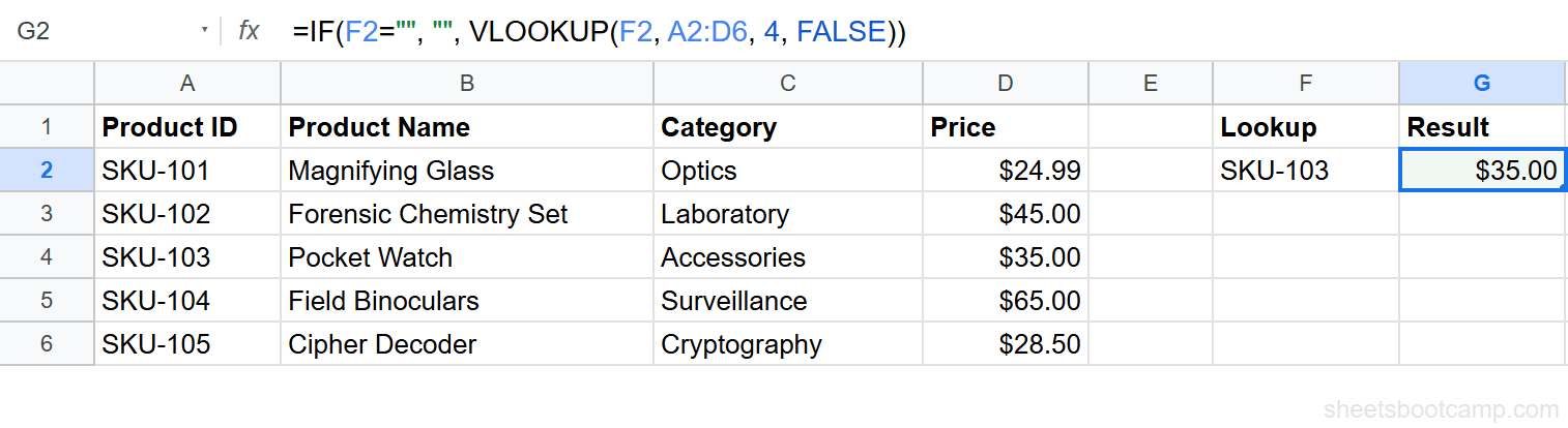
Without the IF wrapper, a blank search cell produces a #N/A error because VLOOKUP cannot find an empty string in your data. The IF check avoids this:
=IF(F2="", "", VLOOKUP(F2, A2:D6, 4, FALSE))| F2 value | Result |
|---|---|
| SKU-103 | $35.00 |
| (empty) | (empty string) |
This formula is a staple for lookup columns where not every row has a search value.
Pattern 2: Use VLOOKUP Result in a Condition
Place VLOOKUP inside the IF condition to make decisions based on the looked-up value:
=IF(VLOOKUP(F2, A2:E6, 5, FALSE)>100, "In Stock", "Low Stock")This looks up the stock quantity for the product in F2. If stock is greater than 100, it returns “In Stock.” Otherwise, “Low Stock.”
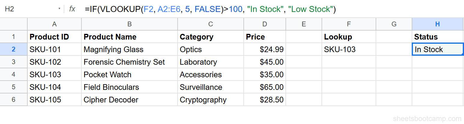
When VLOOKUP is in the IF condition, it runs every time the formula recalculates. If the lookup value does not exist, the formula returns #N/A before IF can evaluate. Wrap the entire formula in IFERROR if missing values are possible.
Pattern 3: Switch Ranges with IF
Use IF inside the VLOOKUP range argument to search different tables based on a condition:
=VLOOKUP(A2, IF(B2="Baker Street", Baker StreetPrices, Scotland YardPrices), 2, FALSE)If column B says “Baker Street,” VLOOKUP searches the Baker StreetPrices named range. Otherwise, it searches Scotland YardPrices.
This pattern is useful when the same product has different prices in different locations, or when data is split across tables by category.
The two ranges must have the same column structure. VLOOKUP uses the same column index regardless of which range IF selects. If one range has the price in column 2 and the other in column 3, the formula returns wrong data.
Pattern 4: Handle Errors with IFERROR
While you can use =IF(ISNA(VLOOKUP(...)), "fallback", VLOOKUP(...)), this runs VLOOKUP twice. IFERROR is the better approach:
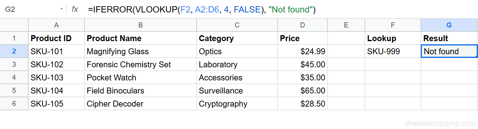
=IFERROR(VLOOKUP(F2, A2:D6, 4, FALSE), "Not found")IFERROR catches any error from VLOOKUP (#N/A, #REF!, #VALUE!) and returns your fallback value. One VLOOKUP call, cleaner syntax.
Combine Patterns: Skip Empty + Handle Errors
For maximum robustness, combine the empty-cell check with IFERROR:
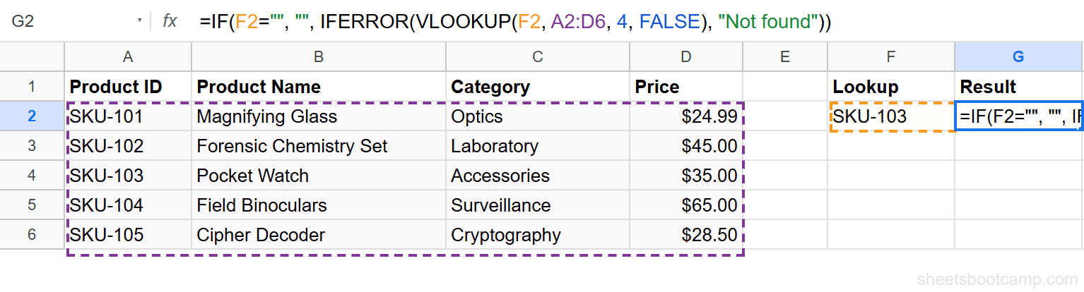
=IF(F2="", "", IFERROR(VLOOKUP(F2, A2:D6, 4, FALSE), "Not found"))This returns blank for empty cells, the price for valid product IDs, and “Not found” for invalid ones.
Step-by-Step: Conditional Lookup
We’ll build a formula that looks up a product price only when the search cell has data, and shows a friendly message when the product is not found.
Set up the lookup with an IF condition
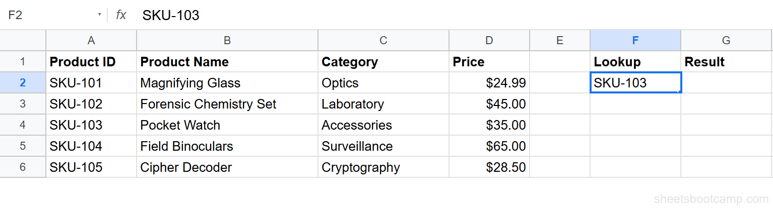
Enter “SKU-103” in cell F2. Column F is where search values go. Column G shows results.
Write the IF-wrapped VLOOKUP formula
Enter the following formula in cell G2:
=IF(F2="", "", IFERROR(VLOOKUP(F2, A2:D6, 4, FALSE), "Not found"))The outer IF checks for an empty cell. IFERROR handles invalid product IDs. VLOOKUP does the actual lookup.
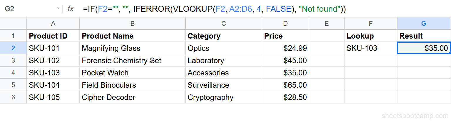
Test with different values
| F2 value | G2 result | Why |
|---|---|---|
| SKU-103 | $35.00 | VLOOKUP found the product |
| (empty) | (empty) | IF caught the blank cell |
| SKU-999 | Not found | IFERROR caught the #N/A |
Copy this formula pattern whenever you build lookup columns. The IF+IFERROR wrapper handles both empty cells and invalid search values, keeping your sheet error-free.
Common Errors and How to Fix Them
#N/A from VLOOKUP Inside IF
The IF condition evaluated to TRUE (the cell is not empty), but VLOOKUP still could not find the value. The IF wrapper does not prevent lookup errors; it only prevents lookups on blank cells.
Fix: Add IFERROR around the VLOOKUP: =IF(F2="", "", IFERROR(VLOOKUP(F2, A2:D6, 4, FALSE), "Not found")).
Formula Returns the VLOOKUP Error Twice
If you use =IF(ISNA(VLOOKUP(...)), "fallback", VLOOKUP(...)), VLOOKUP runs twice. This slows down large sheets and is unnecessary.
Fix: Replace with =IFERROR(VLOOKUP(...), "fallback").
#ERROR! from IF Switching Named Ranges
If the named ranges in the IF condition do not exist or are misspelled, the formula breaks before VLOOKUP runs.
Fix: Verify both named ranges exist in Data > Named ranges. Use the exact range name including capitalization.
Tips and Best Practices
-
Use IFERROR over IF+ISNA. IFERROR is cleaner and runs VLOOKUP only once. The
IF(ISNA(VLOOKUP(...)), ..., VLOOKUP(...))pattern is outdated. -
Always handle empty cells in lookup columns. When the search column has blank rows, wrap VLOOKUP in
IF(cell="", "", VLOOKUP(...))to avoid a column full of#N/Aerrors. -
Nest IFS for multiple conditions. If you need to check several conditions before choosing a lookup approach, IFS is cleaner than deeply nested IF statements.
-
Keep nesting shallow. If your formula has more than three levels of nesting (IF inside IF inside VLOOKUP), consider breaking it into helper columns for readability.
-
Test edge cases. Check your formula with: a valid value, an invalid value, a blank cell, and the first and last values in the range.
Related Google Sheets Tutorials
- VLOOKUP in Google Sheets - Complete guide to VLOOKUP syntax and features
- IF Function in Google Sheets - Full guide to IF statements
- IFERROR Function - Handle errors gracefully in any formula
- Fix VLOOKUP Errors - Troubleshoot #N/A, #REF!, and #VALUE! errors
- Nested IF Statements - Multiple conditions in a single formula
Frequently Asked Questions
Can I use VLOOKUP inside an IF statement?
Yes. Place the VLOOKUP as either the value_if_true or value_if_false argument of IF. For example, =IF(A2<>"", VLOOKUP(A2, data, 2, FALSE), "") runs VLOOKUP only when A2 is not empty.
How do I use IF to handle VLOOKUP errors?
Use IFERROR instead of IF for error handling. =IFERROR(VLOOKUP(A2, B:C, 2, FALSE), "Not found") is cleaner than wrapping VLOOKUP in IF with ISNA or ISERROR.
Can I use IF to choose which range VLOOKUP searches?
Yes. Use IF to switch the range argument: =VLOOKUP(A2, IF(B2="East", EastData, WestData), 2, FALSE). The IF evaluates first, then VLOOKUP searches the selected range.
What is the difference between IFERROR and IF with VLOOKUP?
IFERROR catches any error from VLOOKUP and returns a fallback value. IF with ISNA or ISERROR does the same thing but requires more typing. IFERROR is the preferred approach in Google Sheets.
Can I use VLOOKUP in the condition part of IF?
Yes. Use VLOOKUP as the logical test: =IF(VLOOKUP(A2, B:C, 2, FALSE)>100, "High", "Low"). The VLOOKUP result is compared to 100, and IF returns “High” or “Low” based on the comparison.