AVERAGE, AVERAGEIF, AVERAGEIFS in Google Sheets
Learn how to use AVERAGE, AVERAGEIF, and AVERAGEIFS in Google Sheets. Covers syntax, conditional averages, multiple criteria, and common errors.
Sheets Bootcamp
February 19, 2026 · Updated June 16, 2026
The AVERAGE function in Google Sheets calculates the arithmetic mean of a range of numbers. AVERAGEIF and AVERAGEIFS extend this by averaging only the values that meet one or more conditions — like the average revenue for a specific region or the average salary above a certain threshold.
This guide covers all three functions: AVERAGE for basic means, AVERAGEIF for single-condition averages, and AVERAGEIFS for multiple criteria.
In This Guide
- Syntax and Parameters
- How to Use AVERAGE: Step-by-Step
- AVERAGEIF: Average with One Condition
- AVERAGEIFS: Average with Multiple Conditions
- Practical Examples
- Common Errors and How to Fix Them
- Tips and Best Practices
- Related Google Sheets Tutorials
- FAQ
Syntax and Parameters
AVERAGE
=AVERAGE(value1, [value2], ...)| Parameter | Description | Required |
|---|---|---|
| value1 | A number, cell reference, or range | Yes |
| value2 | Additional values or ranges | No |
AVERAGEIF
=AVERAGEIF(criteria_range, criterion, [average_range])| Parameter | Description | Required |
|---|---|---|
| criteria_range | The range to evaluate against the criterion | Yes |
| criterion | The condition to match (number, text, or expression) | Yes |
| average_range | The range of values to average. If omitted, criteria_range is averaged | No |
AVERAGEIFS
=AVERAGEIFS(average_range, criteria_range1, criterion1, [criteria_range2], [criterion2], ...)| Parameter | Description | Required |
|---|---|---|
| average_range | The range of values to average | Yes |
| criteria_range1 | The first range to evaluate | Yes |
| criterion1 | The condition for criteria_range1 | Yes |
| criteria_range2 | Additional range to evaluate | No |
| criterion2 | The condition for criteria_range2 | No |
AVERAGEIF and AVERAGEIFS have different argument order. In AVERAGEIF, the average_range comes last. In AVERAGEIFS, it comes first. Mixing them up is the most common mistake.
How to Use AVERAGE: Step-by-Step
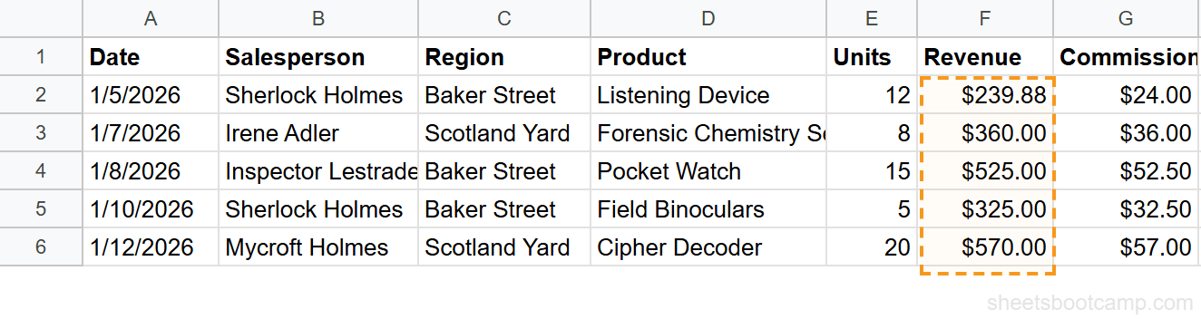
We’ll calculate the average revenue from a sales dataset.
Select the cell for your result
Click cell F21 below the Revenue column. This is where the average will appear.
Enter the AVERAGE formula
Type the formula to average all revenue values:
=AVERAGE(F2:F19)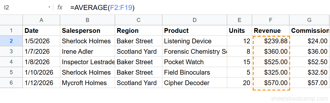
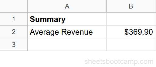
Review the result
The formula returns $369.90, the mean revenue across all 18 sales records. AVERAGE adds up every value in F2:F19 and divides by 18.
AVERAGEIF: Average with One Condition
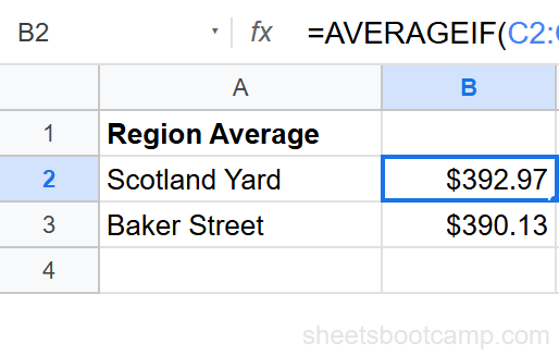
AVERAGEIF calculates the average of values that meet a single condition. Average revenue for a specific region:
=AVERAGEIF(C2:C19, "Scotland Yard", F2:F19)This checks each cell in C2:C19 for “Scotland Yard” and averages the corresponding values in F2:F19. Only the revenue from Scotland Yard sales is included in the calculation.
You can also use comparison operators. Average revenue for sales above 10 units:
=AVERAGEIF(E2:E19, ">10", F2:F19)Comparison operators like ">10" and "<>0" must be wrapped in quotes. Without quotes, Google Sheets interprets them as cell references or math operations instead of conditions.
AVERAGEIFS: Average with Multiple Conditions
AVERAGEIFS works like AVERAGEIF but accepts multiple criteria. All conditions must be true for a value to be included.
Average revenue where region is Baker Street AND units are greater than 10:
=AVERAGEIFS(F2:F19, C2:C19, "Baker Street", E2:E19, ">10")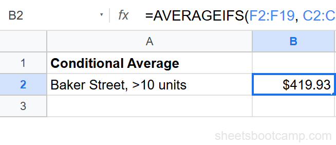
Average salary for employees in the Investigations hired after 2018:
=AVERAGEIFS(F2:F12, C2:C12, "Investigations", D2:D12, ">1/1/2019")Each criteria_range/criterion pair narrows the data further. Only rows matching every condition contribute to the average.
Practical Examples
Average Excluding Zeros
Calculate the average of a range while ignoring zero values:
=AVERAGEIF(F2:F19, "<>0")When average_range is omitted, AVERAGEIF averages the criteria_range itself. The "<>0" criterion excludes zero-value cells from the calculation.
Average by Salesperson
Average commission earned by Sherlock Holmes:
=AVERAGEIF(B2:B19, "Sherlock Holmes", G2:G19)This returns the mean commission across all of Fred’s sales records. Combine with SUMIF to get the total instead.
Weighted Average (Manual)
Google Sheets doesn’t have a WEIGHTEDAVERAGE function. Calculate it with SUMPRODUCT and SUM:
=SUMPRODUCT(E2:E19, F2:F19) / SUM(E2:E19)This multiplies each unit count by its revenue, sums the products, then divides by total units — giving a units-weighted average revenue.
Common Errors and How to Fix Them
#DIV/0! Error
No values match the criteria (AVERAGEIF/AVERAGEIFS), or the range contains no numbers (AVERAGE). Check your criterion for typos. If the condition legitimately might match zero rows, wrap in IFERROR: =IFERROR(AVERAGEIF(C2:C19, "North", F2:F19), 0).
#VALUE! Error
The ranges in AVERAGEIFS are different sizes. All criteria_range and average_range arguments must have the same number of rows. Check that your ranges match: F2:F19 (18 rows) paired with C2:C19 (18 rows), not C2:C20 (19 rows).
Wrap AVERAGEIF in IFERROR when the criteria might match zero rows: =IFERROR(AVERAGEIF(C2:C19, "North", F2:F19), "No data"). This prevents #DIV/0! from appearing in dashboards and reports.
Wrong Result (Includes Text Cells)
AVERAGE ignores text cells, but a cell containing “100” as text (not a number) is skipped. If your average seems too low, check that number cells are formatted as numbers. Select the range and go to Format > Number to verify.
Tips and Best Practices
-
AVERAGE ignores blanks but includes zeros. An empty cell doesn’t affect the average, but a cell containing 0 does. Use AVERAGEIF with
"<>0"when zeros should be excluded. -
Use AVERAGEIFS for date ranges. Combine two date criteria:
=AVERAGEIFS(F2:F19, A2:A19, ">=1/1/2026", A2:A19, "<=1/31/2026")to average January values only. -
Wildcards work in AVERAGEIF. Use
*for any characters and?for a single character:=AVERAGEIF(D2:D19, "Ext*", F2:F19)averages revenue for all products starting with “Ext”. -
Pair with COUNTIF for context. Showing an average without the count can be misleading. Display both: “Average: $450 (based on 5 records)” gives the reader confidence in the number.
-
Use SUBTOTAL for filtered data.
=SUBTOTAL(101, F2:F19)averages only visible cells. Regular AVERAGE includes hidden rows, which produces wrong results when filters are active.
Related Google Sheets Tutorials
- SUMIF and SUMIFS in Google Sheets - Sum values by condition instead of averaging them
- COUNTIF and COUNTIFS in Google Sheets - Count how many values match a condition
- COUNT, COUNTA, COUNTBLANK - Count cells by type (numbers, non-empty, blanks)
- MAX, MIN, LARGE, and SMALL - Find the highest and lowest values in a range
FAQ
How do I calculate an average in Google Sheets?
Use =AVERAGE(range) where range is the cells containing numbers. For example, =AVERAGE(B2:B50) returns the arithmetic mean of all numeric values in B2 through B50. The function ignores text and empty cells.
What is the difference between AVERAGE and AVERAGEIF?
AVERAGE calculates the mean of all numbers in a range. AVERAGEIF calculates the mean of only the numbers that meet a specific condition. For example, =AVERAGEIF(A2:A10, “North”, B2:B10) averages values in column B only where column A equals North.
How do I use AVERAGEIFS with multiple criteria?
Use =AVERAGEIFS(average_range, criteria_range1, criterion1, criteria_range2, criterion2). For example, =AVERAGEIFS(F2:F19, C2:C19, “Scotland Yard”, E2:E19, “>10”) averages revenue where region is Scotland Yard AND units are greater than 10.
Does AVERAGE ignore blank cells?
Yes. AVERAGE skips blank cells and text values entirely. A cell containing 0 is included in the calculation, but an empty cell is not. This means blank cells do not lower your average.
How do I average only visible cells in Google Sheets?
Use =SUBTOTAL(101, range) instead of AVERAGE. The SUBTOTAL function with function number 101 calculates the average of only visible cells, ignoring rows hidden by filters.
Why does AVERAGE return #DIV/0!?
The range contains no numeric values. If every cell in the range is blank, text, or an error, AVERAGE has nothing to divide and returns #DIV/0!. Check that your range contains at least one number.