How to Reference Another Sheet in Google Sheets
Learn how to reference cells and ranges from another sheet tab in Google Sheets. Covers the exclamation point syntax, spaces in sheet names, and formulas.
Sheets Bootcamp
March 15, 2026 · Updated April 4, 2026
A sheet reference in Google Sheets lets you pull data from one tab into another tab within the same spreadsheet. The syntax uses an exclamation point between the sheet name and the cell: Products!B2 means “cell B2 on the Products sheet.”
This comes up any time you organize data across multiple tabs. You might keep raw data on one sheet and build a summary on another, or store product details in one place and reference them from an order tracker. This guide covers the syntax, step-by-step examples, and how to use sheet references inside formulas like VLOOKUP and SUM.
In This Guide
- How Sheet References Work
- How to Reference a Cell in Another Sheet: Step-by-Step
- Reference a Range from Another Sheet
- Sheet Names with Spaces
- Using Sheet References in Formulas
- Reference a Different Spreadsheet File
- Common Mistakes and Fixes
- Tips and Best Practices
- Related Google Sheets Tutorials
- FAQ
How Sheet References Work
Every cell in Google Sheets has an address that includes the sheet name and the cell coordinate. When you work on a single sheet, you only type the cell part: A1, B2:D10. When you reference a cell on a different sheet, you add the sheet name and an exclamation point in front.
The format is:
=SheetName!CellReferenceFor example, =Products!B2 returns the value of cell B2 from the sheet named “Products.” The exclamation point is the separator. Everything before it is the sheet name. Everything after it is the cell or range.
| Syntax | Meaning |
|---|---|
=Products!B2 | Cell B2 on the Products sheet |
=Products!A1:D10 | Range A1:D10 on the Products sheet |
='Product List'!B2 | Cell B2 on a sheet named “Product List” (quotes needed for spaces) |
Sheet references only work within the same spreadsheet file. To pull data from a different Google Sheets file, you need the IMPORTRANGE function.
How to Reference a Cell in Another Sheet: Step-by-Step
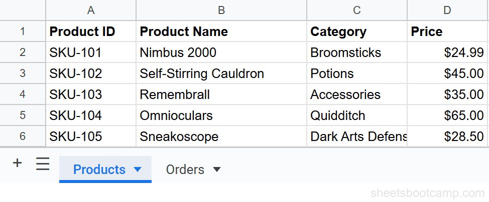
Start with a spreadsheet that has two sheet tabs. In this example, the “Products” sheet holds a product inventory with IDs, names, categories, and prices.
Click the Orders tab to switch to the second sheet. This is where you will pull data from Products.
On the Orders sheet, click cell B2. Type the following formula:
=Products!B2The sheet name (Products) goes first, then the exclamation point, then the cell address (B2). Press Enter.
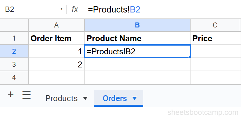
You can also type = then click the Products tab, click cell B2, and press Enter. Google Sheets builds the reference for you. This is faster and avoids typos in the sheet name.
Cell B2 now displays “Nimbus 2000,” the product name from cell B2 on the Products sheet. Click the cell to confirm the formula bar shows =Products!B2.

The value updates automatically. If someone changes the product name on the Products sheet, the Orders sheet reflects the change immediately.
Reference a Range from Another Sheet
Single-cell references are useful, but you can also reference an entire range. This is how you use data from another sheet inside aggregate formulas like SUM, AVERAGE, or COUNT.
To add up all the prices on the Products sheet:
=SUM(Products!D2:D6)This adds cells D2 through D6 on the Products sheet and returns the total.
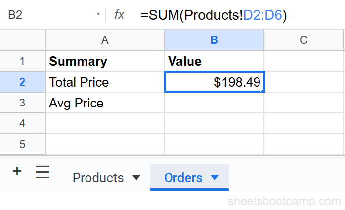
The same pattern works with any function that accepts a range: =AVERAGE(Products!D2:D6), =COUNT(Products!A2:A6), =MAX(Products!D2:D6).
Sheet Names with Spaces
If a sheet name contains spaces, you must wrap it in single quotes. Without quotes, Google Sheets cannot tell where the sheet name ends.
='Product List'!B2The single quotes go around the sheet name only, not around the entire reference. The exclamation point and cell address stay outside the quotes.
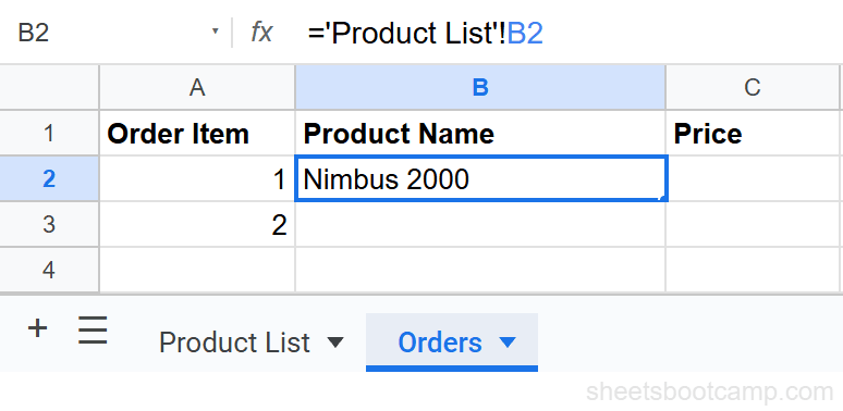
When you click a cell on another sheet to build the reference, Google Sheets adds single quotes automatically if the sheet name has spaces. You only need to type them manually when entering the reference by hand.
Special characters in sheet names (hyphens, periods, parentheses) also require single quotes. The safest approach: keep sheet names short, descriptive, and free of spaces. Products is easier to reference than Product List (2026).
Using Sheet References in Formulas
Sheet references work inside any formula. The sheet name becomes part of the range argument.
VLOOKUP with another sheet
To look up a product price from the Products sheet while working on the Orders sheet:
=VLOOKUP(A2,Products!A2:D6,4,FALSE)This searches for the value in A2 (a Product ID like “SKU-103”) in the first column of the Products range, and returns the price from column 4.
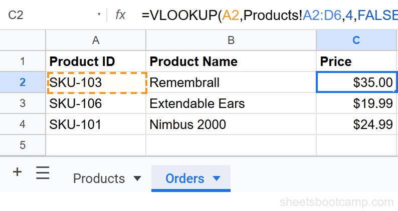
For a full walkthrough of this pattern, see VLOOKUP from Another Sheet.
SUMIF with another sheet
To sum prices for a specific category on the Products sheet:
=SUMIF(Products!C2:C6,'Quidditch',Products!D2:D6)The criteria range and sum range both reference the Products sheet. The criteria (“Quidditch”) is a text string. For more on this pattern, see the SUMIF and SUMIFS guide.
When copying formulas that reference another sheet, use absolute references ($ signs) on the range if it should stay fixed. Products!$A$2:$D$6 keeps the range locked as you copy the formula to other cells.
Reference a Different Spreadsheet File
Sheet tab references like Products!B2 only work within the same Google Sheets file. If you need data from a completely separate spreadsheet, use IMPORTRANGE.
=IMPORTRANGE("spreadsheet_url","Products!A1:D10")IMPORTRANGE connects two different files. The first argument is the URL of the source spreadsheet. The second is the sheet name and range, formatted as a text string.
The first time you use IMPORTRANGE with a new source file, Google Sheets asks you to grant access permission. After that, the data flows automatically. See the IMPORTRANGE guide for the full setup.
Common Mistakes and Fixes
#REF! error after deleting a sheet
If you delete or remove the sheet that a formula references, every formula pointing to it shows #REF!. The formula bar displays something like =#REF!B2.

The fix: undo the deletion (Ctrl+Z) or recreate the sheet with the exact same name. Google Sheets updates references automatically when you rename a sheet, but deleting it breaks the link permanently.
Missing quotes around sheet names with spaces
If the formula bar shows an error and your sheet name has a space, check for single quotes. =Product List!B2 breaks. ='Product List'!B2 works. Google Sheets usually adds quotes when you click to build the reference, but manually typed references are easy to get wrong.
Wrong sheet name (typo)
If you mistype the sheet name, Google Sheets shows a parsing error. Double-check the tab name. Sheet names are case-sensitive in some contexts, so match the capitalization exactly, or click the tab to let Google Sheets insert the name for you.
Tips and Best Practices
-
Click to build references instead of typing. Type
=in the destination cell, click the source sheet tab, click the cell, and press Enter. This avoids typos and automatically adds quotes for sheet names with spaces. -
Keep sheet names short and without spaces.
Productsis easier to reference thanProduct Inventory (Main). Shorter names mean shorter formulas and fewer quoting issues. -
Use absolute references when copying. If you copy a formula that references another sheet’s range, add
$signs to lock the range:Products!$A$2:$D$6. Without them, the range shifts as you paste, which can return wrong results. -
Rename sheets freely. Google Sheets automatically updates all formulas that reference a renamed sheet. Renaming
Sheet1toProductsupdates every=Sheet1!B2reference to=Products!B2throughout the file. -
For cross-file references, use IMPORTRANGE. The
SheetName!Cellsyntax only works within the same file. If you find yourself trying to reference a sheet that does not appear in your tab list, you likely need IMPORTRANGE instead.
Related Google Sheets Tutorials
- VLOOKUP: The Complete Guide - Lookup formulas frequently use cross-sheet ranges as the data source
- VLOOKUP from Another Sheet - Step-by-step guide to using VLOOKUP with data on a different tab
- IMPORTRANGE: The Complete Guide - Pull data from a different Google Sheets file into your current spreadsheet
- Absolute vs Relative References - Lock cell references with the
$sign when copying formulas - SUMIF and SUMIFS - Conditionally sum data, including data on other sheets
FAQ
How do I reference another sheet in Google Sheets?
Type the sheet name followed by an exclamation point and the cell reference. For example, =Sheet2!A1 pulls the value from cell A1 on Sheet2. If the sheet name has spaces, wrap it in single quotes: ='Sheet Name'!A1.
What does the exclamation point mean in a Google Sheets formula?
The exclamation point separates the sheet name from the cell reference. In =Products!B2, the exclamation point tells Google Sheets to look for cell B2 on the sheet named Products.
How do I reference a range from another sheet?
Use the same syntax with a range instead of a single cell. For example, =SUM(Products!D2:D6) adds the values in cells D2 through D6 on the Products sheet.
Do I need quotes around the sheet name?
Only if the sheet name contains spaces or special characters. Products!A1 works without quotes. 'Product List'!A1 needs single quotes because the name has a space. Google Sheets adds the quotes automatically if you click to select the cell.
How do I reference a cell from a different Google Sheets file?
Use the IMPORTRANGE function. Sheet tab references (like Products!A1) only work within the same spreadsheet file. To pull data from a separate file, use =IMPORTRANGE("spreadsheet_url", "Sheet1!A1:C10").
What happens if I rename a sheet that other formulas reference?
Google Sheets updates the references automatically. If you rename “Products” to “Inventory,” any formula that said =Products!B2 changes to =Inventory!B2. Deleting the sheet, however, causes a #REF! error.