IF Statement with Checkbox in Google Sheets

An IF checkbox formula in Google Sheets returns a custom value based on whether a checkbox is checked or unchecked. Checkboxes store TRUE or FALSE, and the IF function reads that value to produce a label, trigger a calculation, or flag a status. This is useful for task trackers, to-do lists, and approval workflows where you need a formula that reacts when someone ticks a box. We’ll cover how checkboxes work, walk through a step-by-step example, and show practical formulas you can use right away.

In This Guide

• How Checkboxes Work in Google Sheets
• IF with Checkbox: Step-by-Step
• Practical Examples
• Common Errors and How to Fix Them
• Tips and Best Practices
• Related Google Sheets Tutorials
• FAQ

How Checkboxes Work in Google Sheets

A checkbox in Google Sheets is a cell that stores a boolean value. Checked equals TRUE. Unchecked equals FALSE. You can confirm this by selecting any checkbox cell and looking at the formula bar.

You insert checkboxes through Data > Data validation > Criteria > Checkbox. This is covered in detail in the checkbox data validation guide. For this article, what matters is the underlying value: TRUE or FALSE.

Because IF already evaluates boolean values, you can reference a checkbox cell directly as the logical test:

=IF(F2, "Done", "Pending")

No need to write =IF(F2=TRUE, "Done", "Pending"). The IF function checks whether its first argument is TRUE or FALSE. A checkbox cell is already TRUE or FALSE, so the shorter syntax works. The longer F2=TRUE version also works and some people find it more readable. Both produce the same result.

IF with Checkbox: Step-by-Step

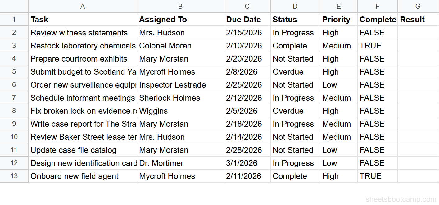
We’ll use a task tracker with 12 rows. Column F (Complete) contains checkboxes. Two tasks are checked: “Restock laboratory chemicals” (row 2) and “Onboard new field agent” (row 13). We’ll add an IF formula in column G to display “Done” or “Pending” based on each checkbox.

Open the spreadsheet with task data in columns A through F. Column F has checkboxes. Two tasks show checked boxes (TRUE), and ten show unchecked boxes (FALSE). Column G is empty and ready for the formula.

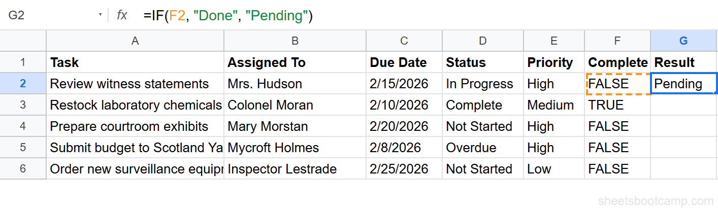
Select cell G2. Enter the formula:

=IF(F2, "Done", "Pending")

Press Enter. Cell F2 is unchecked (FALSE), so G2 displays “Pending”.

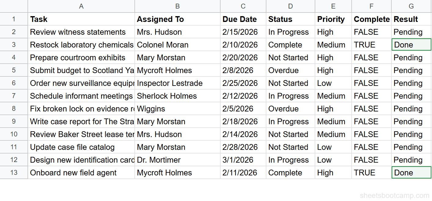
Copy G2 down through G13. Each cell reads the checkbox in its row. Two cells display “Done”:

• G3 (Restock laboratory chemicals) — checkbox is checked
• G13 (Onboard new field agent) — checkbox is checked

The remaining ten cells display “Pending”.

Click the checkbox in cell F4 to check it. Cell G4 immediately changes from “Pending” to “Done”. Click the checkbox again to uncheck it. G4 returns to “Pending”. The IF formula reacts in real time because the cell value changes from FALSE to TRUE and back.

Practical Examples

Count Completed Tasks with COUNTIF

You can count how many checkboxes are checked without writing an IF formula for each row. COUNTIF counts cells matching a condition directly.

=COUNTIF(F2:F13, TRUE)

This returns 2, matching the two checked boxes in the task tracker. To count unchecked boxes, use:

=COUNTIF(F2:F13, FALSE)

This returns 10. You can use these counts to build a progress summary. For example, to show a completion percentage:

=COUNTIF(F2:F13, TRUE) / COUNTA(F2:F13)

This divides checked tasks (2) by total tasks (12), returning approximately 0.167. Format the cell as a percentage to display 17%.

IF Checkbox with AND for Multiple Conditions

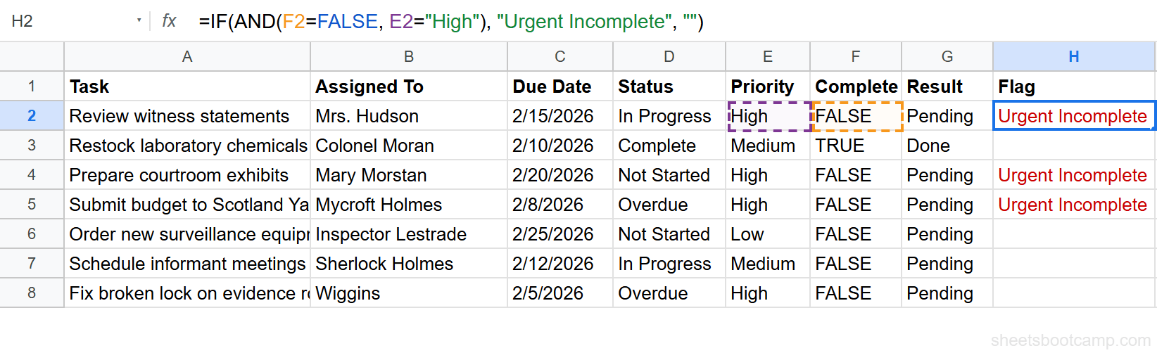
Combine a checkbox check with another condition using IF with AND. Here we want to label a task as “Urgent Incomplete” when the checkbox is unchecked AND the priority is “High”.

=IF(AND(F2=FALSE, E2="High"), "Urgent Incomplete", "")

This checks two things: the checkbox in column F is unchecked, and the priority in column E is “High”. Three tasks match: “Review witness statements” (row 2), “Prepare courtroom exhibits” (row 4), and “Submit budget to Scotland Yard” (row 5). The remaining cells return an empty string.

Trigger Conditional Formatting from Checkboxes

You can highlight entire rows based on checkbox status using conditional formatting. Select the data range A2:G13. Add a custom formula rule:

=$F2=TRUE

Set the format to a green background. Every row with a checked box gets highlighted. The dollar sign locks the column reference to F while the row number adjusts for each row.

This pairs well with the IF formula in column G. The checkbox drives both the cell label and the visual formatting.

Common Errors and How to Fix Them

Text “TRUE” Instead of Boolean TRUE

The most common issue. If someone types the word TRUE into a cell instead of inserting a checkbox, the cell contains a text string, not a boolean value. Text “TRUE” looks identical in the cell, but IF may not evaluate it the same way.

How to spot it: Select the cell and check the formula bar. A boolean TRUE appears without quotes. A text “TRUE” may appear the same, but the checkbox toggle won’t be present.

Fix: Delete the cell contents. Go to Data > Data validation and insert a proper checkbox. The cell now stores a real boolean value.

Referencing the Wrong Cell

If your IF formula returns “Done” when the checkbox is unchecked, the formula is reading a different cell than you expect. This happens when the formula references the wrong column or has an absolute reference that doesn’t adjust when copied down.

Fix: Select the formula cell and check the formula bar. Confirm the reference points to the checkbox column (F in our example). Make sure the row reference is relative (F2, not $F$2) so it updates when you copy the formula down.

Checkbox Not Inserted via Data Validation

Typing TRUE or FALSE manually creates a value that looks like a checkbox state but has no toggle. The cell works with IF formulas, but the user cannot click to check or uncheck it.

Fix: Select the cells where you need checkboxes. Go to Data > Data validation > Add rule. Under Criteria, select Checkbox. Click Done. The cells now display clickable checkboxes that toggle between TRUE and FALSE.

Tips and Best Practices

1. Use the short syntax. Write =IF(F2, "Done", "Pending") instead of =IF(F2=TRUE, "Done", "Pending"). Both work, but the short version is cleaner. IF already evaluates TRUE/FALSE natively.

2. Combine with SUMIF for conditional totals. If column D has hours and column F has checkboxes, =SUMIF(F2:F13, TRUE, D2:D13) adds up hours for completed tasks only. No IF formula needed per row.

3. Nest IF for multiple outcomes. Use a nested IF to return three states: =IF(F2, "Complete", IF(E2="High", "Urgent", "Pending")). This labels checked tasks as “Complete”, unchecked high-priority tasks as “Urgent”, and everything else as “Pending”.

4. Lock the checkbox column in shared sheets. If multiple people edit the sheet, protect column G (the formula column) so users can only toggle checkboxes in column F. Go to Data > Protect sheets and ranges to set permissions.

5. Use ARRAYFORMULA for the entire column. Instead of copying the formula down manually, enter one formula in G2: =ARRAYFORMULA(IF(F2:F13, "Done", "Pending")). This fills G2:G13 with a single formula.

Related Google Sheets Tutorials

• IF Function in Google Sheets: Complete Guide - Full syntax breakdown and all logical operators for the IF function
• Checkbox in Google Sheets - How to insert, customize, and manage checkboxes with data validation
• Nested IF in Google Sheets - Build multi-level decision logic with nested IF formulas
• IF with AND and OR in Google Sheets - Combine checkboxes with other conditions using AND and OR
• Conditional Formatting in Google Sheets - Highlight rows based on checkbox status with formula-based rules

FAQ

Does a checkbox in Google Sheets return TRUE or FALSE?

Yes. A checked box stores the boolean value TRUE in the cell. An unchecked box stores FALSE. You can verify this by selecting a checkbox cell and looking at the formula bar.

Do I need to write IF(F2=TRUE) or can I use IF(F2)?

Both work. IF already evaluates TRUE or FALSE, so =IF(F2, “Done”, “Pending”) is equivalent to =IF(F2=TRUE, “Done”, “Pending”). The shorter version is cleaner, but the longer version is more readable if you prefer explicit comparisons.

Why does my IF formula return the wrong result for a checkbox?

The most common cause is that the cell contains the text string “TRUE” instead of the boolean value TRUE. Text TRUE looks the same but is not a real boolean. Delete the cell contents, then insert a checkbox through Data > Data validation to get a proper boolean value.

Can I count how many checkboxes are checked in Google Sheets?

Yes. Use =COUNTIF(F2:F13, TRUE) to count every checked box in the range F2:F13. COUNTIF treats the boolean TRUE as a match, so it counts only the checked cells.

How do I use a checkbox with conditional formatting?

Create a conditional formatting rule with a custom formula. Select the row range, set the formula to =F2=TRUE (adjusting the column to your checkbox column), and choose a format like a green background. The formatting applies automatically when the checkbox is checked.