Text Functions in Google Sheets: Complete Guide
Learn how to use text functions in Google Sheets to clean, combine, and extract data. Covers TRIM, PROPER, SPLIT, SUBSTITUTE, and more with examples.
Sheets Bootcamp
February 18, 2026
Text functions in Google Sheets clean, extract, combine, and transform the text in your cells. Imported data from forms, CRMs, or CSV files almost always arrives with extra spaces, inconsistent capitalization, or formatting that needs fixing. Text functions handle that cleanup without manual editing.
This guide covers the most useful Google Sheets text formulas, walks through cleaning a messy contacts list step by step, and shows practical examples for extracting, combining, and standardizing text data.
In This Guide
- What Are Text Functions in Google Sheets?
- Essential Text Functions: Syntax and Examples
- How to Clean Messy Data: Step-by-Step
- Text Function Examples
- Combining Text Functions
- Common Errors and How to Fix Them
- Tips and Best Practices
- Related Google Sheets Tutorials
- FAQ
What Are Text Functions in Google Sheets?
Text functions are formulas that work on text strings rather than numbers. They let you change case, remove whitespace, extract portions of a string, find characters, combine values from multiple cells, and replace text with formulas instead of manual editing.
Google Sheets has over 30 text functions. Some fix formatting problems (TRIM, CLEAN, UPPER, LOWER, PROPER). Some extract parts of a string (LEFT, RIGHT, MID). Some combine text from multiple cells (CONCATENATE, TEXTJOIN, the & operator). And some find or replace characters within a string (FIND, SEARCH, SUBSTITUTE).
Text functions are especially useful for cleaning imported data. A CSV export from a CRM might have names in ALL CAPS, extra spaces between words, or email addresses in mixed case. Instead of fixing 500 rows by hand, one formula handles the entire column.
For the official list of text functions, see Google’s function reference.
Essential Text Functions: Syntax and Examples
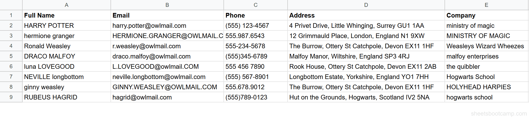
We’ll use a messy contacts list throughout this section. The data has names with extra spaces and inconsistent capitalization, emails in mixed case, and company names that need standardizing.
TRIM and CLEAN
TRIM removes leading spaces, trailing spaces, and collapses multiple spaces between words down to one.
=TRIM(text)CLEAN removes non-printable characters (characters with ASCII codes 0 through 31) that sometimes appear in imported data.
=CLEAN(text)Example: Cell A3 contains " Ronald Weasley " with leading and trailing spaces. =TRIM(A3) returns "Ronald Weasley" with all extra spaces removed.
For data imported from web pages or external systems, combine them: =TRIM(CLEAN(A3)) strips both invisible characters and extra whitespace. For a deeper look at edge cases, see the TRIM and CLEAN guide.
UPPER, LOWER, PROPER
These three functions change the capitalization of text.
=UPPER(text)=LOWER(text)=PROPER(text)- UPPER converts every letter to uppercase.
=UPPER("harry potter")returns"HARRY POTTER". - LOWER converts every letter to lowercase.
=LOWER("HERMIONE.GRANGER@OWLMAIL.COM")returns"hermione.granger@owlmail.com". - PROPER capitalizes the first letter of each word.
=PROPER("ministry of magic")returns"Ministry Of Magic".
Example: Cell A1 contains "HARRY POTTER". =PROPER(A1) returns "Harry Potter" — note that PROPER fixes the case but does not remove the extra spaces. You need TRIM for that.
For all three functions with edge cases and mixed-case handling, see the UPPER, LOWER, PROPER guide.
PROPER capitalizes the first letter after every space, hyphen, or punctuation mark. This means =PROPER("o'brien") returns "O'Brien" — which is correct. But =PROPER("mcdonalds") returns "Mcdonalds" — not "McDonalds". PROPER does not recognize capitalization patterns within words.
LEFT, RIGHT, MID
These functions extract a specific number of characters from a text string.
=LEFT(text, num_characters)=RIGHT(text, num_characters)=MID(text, start_position, num_characters)- LEFT pulls characters from the beginning.
=LEFT("Harry Potter", 5)returns"Harry". - RIGHT pulls characters from the end.
=RIGHT("GU1 1AA", 3)returns"1AA". - MID pulls characters from any position.
=MID("(555) 123-4567", 2, 3)returns"555".
Example: To extract the area code from "(555) 123-4567" in cell C1, use =MID(C1, 2, 3). This starts at position 2 (skipping the opening parenthesis) and pulls 3 characters, returning "555".
For more extraction patterns, see the LEFT, RIGHT, MID guide.
CONCATENATE and the & Operator
CONCATENATE joins two or more text strings into one. The & operator does the same thing with shorter syntax.
=CONCATENATE(string1, string2, ...)Example: To build a greeting from a name, =CONCATENATE("Hello, ", A2) returns "Hello, HARRY POTTER" when A2 contains "HARRY POTTER". You can also write ="Hello, " & A2 for the same result.
The & operator is more common in practice because it’s shorter to type. =A2 & " - " & E2 joins a name and company with a dash between them.
CONCATENATE does not add spaces between values automatically. If you write =CONCATENATE(A2, B2), the two values run together with no space. Add a space string between them: =CONCATENATE(A2, " ", B2), or use TEXTJOIN with a delimiter instead.
TEXTJOIN
TEXTJOIN joins a range of cells with a delimiter you choose. It also has an option to skip empty cells.
=TEXTJOIN(delimiter, ignore_empty, string1, [string2, ...])| Argument | Description | Required |
|---|---|---|
| delimiter | Text placed between each value (e.g., ", " or " - ") | Yes |
| ignore_empty | TRUE to skip blank cells, FALSE to include them | Yes |
| string1 | First value or range to join | Yes |
Example: =TEXTJOIN(", ", TRUE, "Harry", "Potter", "London") returns "Harry, Potter, London". When referencing a range: =TEXTJOIN(" | ", TRUE, A2:E2) joins all five columns in row 2 with a pipe separator.
TEXTJOIN is more flexible than CONCATENATE because it accepts ranges and handles empty cells. For joining patterns and advanced delimiters, see the CONCATENATE and TEXTJOIN guide.
SPLIT
SPLIT breaks a text string into separate cells at each occurrence of a delimiter.
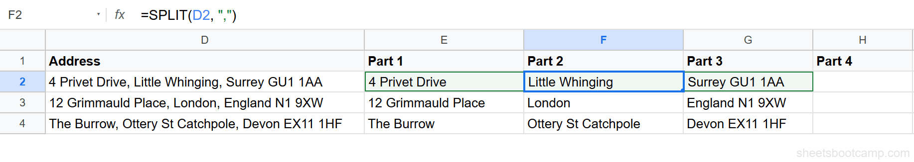
=SPLIT(text, delimiter, [split_by_each], [remove_empty])Example: Cell D1 contains "4 Privet Drive, Little Whinging, Surrey GU1 1AA". =SPLIT(D1, ",") splits this into four cells: "4 Privet Drive", " Little Whinging", " Surrey GU1 1AA".
Set the third argument to FALSE to treat the entire delimiter as one string rather than splitting at each character individually. For more SPLIT patterns, see the SPLIT function guide.
SPLIT outputs to adjacent cells to the right. If those cells contain data, SPLIT returns a #REF! error instead of overwriting them. Clear the cells to the right before using SPLIT, or place the formula in an empty area.
SUBSTITUTE
SUBSTITUTE replaces specific text within a string. Unlike Find and Replace (Ctrl+H), SUBSTITUTE works inside formulas and can target a specific occurrence.
=SUBSTITUTE(text, old_text, new_text, [occurrence])Example: To standardize phone numbers, =SUBSTITUTE(C4, "(555)", "555") changes "(555)345-6789" to "555345-6789". You can chain multiple SUBSTITUTE calls to remove parentheses, dashes, and dots: =SUBSTITUTE(SUBSTITUTE(SUBSTITUTE(C2, "(", ""), ")", ""), "-", "").
For more replacement patterns and chaining strategies, see the SUBSTITUTE guide.
LEN
LEN returns the number of characters in a text string, including spaces.
=LEN(text)Example: =LEN("HARRY POTTER") returns 14 because it counts every character including the three spaces. =LEN(TRIM("HARRY POTTER")) returns 12 because TRIM collapses the three spaces to one.
LEN is useful for validating data. Combine it with conditional formatting to highlight cells where text exceeds a character limit, or use it with IF statements to flag entries that are too short or too long.
FIND and SEARCH
FIND and SEARCH both locate the position of one text string within another. The key difference: FIND is case-sensitive, SEARCH is not.
=FIND(search_for, text_to_search, [starting_at])=SEARCH(search_for, text_to_search, [starting_at])Example: =FIND("P", "Harry Potter") returns 7 because the uppercase P is at position 7. =FIND("p", "Harry Potter") returns an error because there is no lowercase p. =SEARCH("p", "Harry Potter") returns 7 because SEARCH ignores case.
FIND and SEARCH are most useful combined with LEFT, RIGHT, or MID to extract text dynamically. Instead of hardcoding how many characters to extract, you use FIND to locate a delimiter and calculate the count. For patterns and examples, see the FIND and SEARCH guide.
How to Clean Messy Data: Step-by-Step
We’ll clean a contacts list that has names with extra spaces, inconsistent capitalization, mixed-case emails, and messy company names. The table has 8 contacts with columns for Full Name, Email, Phone, Address, and Company.
Examine the messy data
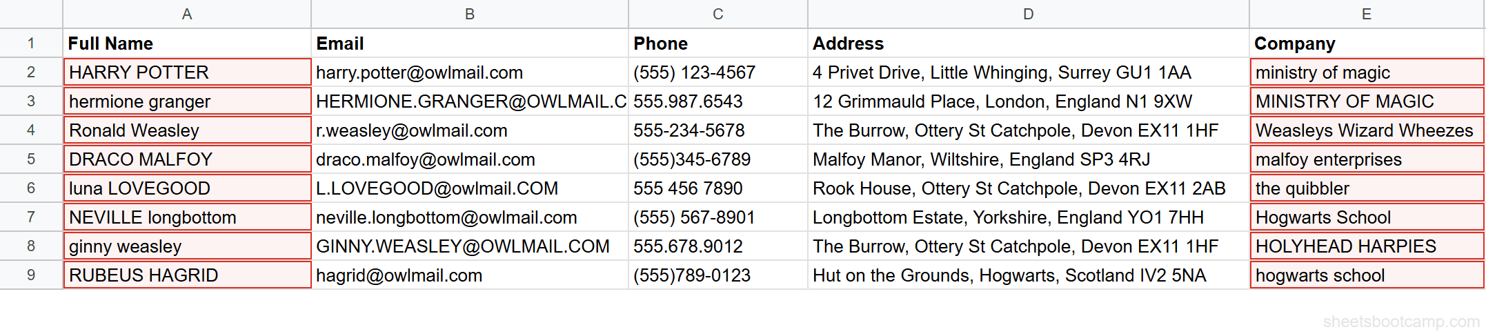
Open the contacts spreadsheet. The problems are visible immediately: "HARRY POTTER" has extra spaces and is all caps. "hermione granger" is all lowercase. " Ronald Weasley " has leading and trailing spaces. "luna LOVEGOOD" has mixed case. Company names range from "ministry of magic" to "HOLYHEAD HARPIES".
Remove extra spaces with TRIM
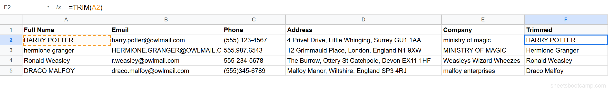
Select cell F2 and enter the formula:
=TRIM(A2)This removes the extra spaces from the Full Name column. "HARRY POTTER" becomes "HARRY POTTER". " Ronald Weasley " becomes "Ronald Weasley". Copy the formula down through F9 for all 8 rows.
After copying TRIM formulas down a column, you can paste the cleaned values over the original data using Paste special > Values only (Ctrl+Shift+V). This replaces the messy text with the clean version and removes the formula dependency.
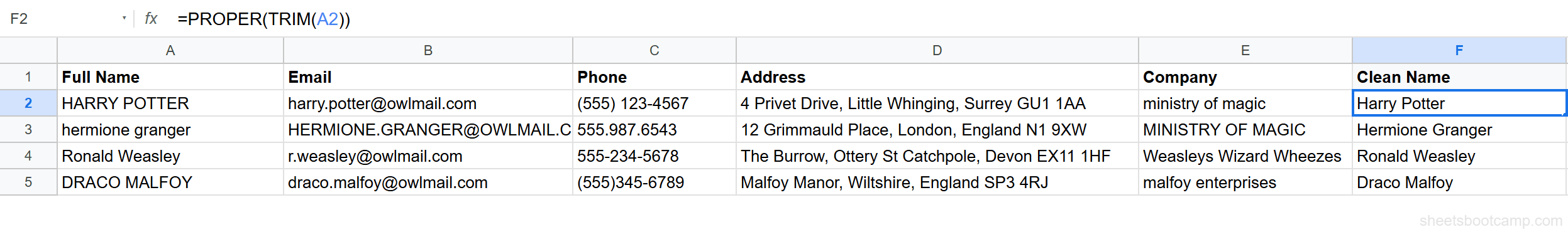
Fix capitalization with PROPER
Nest TRIM inside PROPER to handle both spacing and capitalization in one formula. Select cell G2 and enter:
=PROPER(TRIM(A2))This cleans the name and converts it to proper case in one step. "HARRY POTTER" becomes "Harry Potter". " NEVILLE longbottom " becomes "Neville Longbottom". "luna LOVEGOOD" becomes "Luna Lovegood".
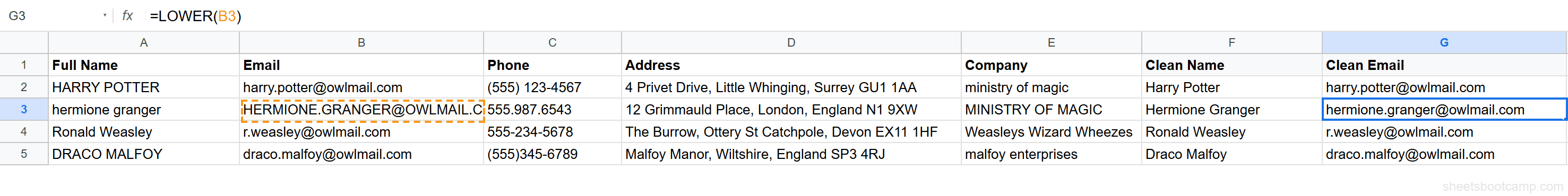
Standardize emails with LOWER
Email addresses should always be lowercase. Select cell H2 and enter:
=LOWER(B2)"HERMIONE.GRANGER@OWLMAIL.COM" becomes "hermione.granger@owlmail.com". "L.LOVEGOOD@owlmail.COM" becomes "l.lovegood@owlmail.com". "GINNY.WEASLEY@OWLMAIL.COM" becomes "ginny.weasley@owlmail.com".
Clean company names
Company names need the same treatment as names. Select cell I2 and enter:
=TRIM(PROPER(E2))"ministry of magic" becomes "Ministry Of Magic". "HOLYHEAD HARPIES" becomes "Holyhead Harpies". "hogwarts school" becomes "Hogwarts School". "malfoy enterprises" becomes "Malfoy Enterprises".
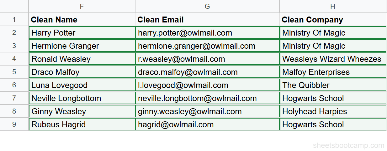
The contacts list is now consistent. Names are properly capitalized with no extra spaces, emails are lowercase, and company names follow the same format.
Text Function Examples
Example 1: Extract First Name with LEFT and FIND
You need a first name column from the full name. The first name is everything before the first space.
=LEFT(A2, FIND(" ", A2) - 1)FIND locates the position of the first space. Subtracting 1 gives the number of characters in the first name. LEFT extracts that many characters from the start.
For "Harry Potter" in A2, FIND(" ", A2) returns 6. LEFT(A2, 6 - 1) returns "Harry". For "Luna Lovegood", FIND returns 5, and LEFT returns "Luna".
This formula breaks if the name has no space — a single-word name like "Hagrid" causes FIND to return an error. Wrap it in IFERROR to handle that case: =IFERROR(LEFT(A2, FIND(" ", A2) - 1), A2). This returns the full cell value when no space exists.
Example 2: Standardize Phone Numbers
The contacts have phone numbers in four different formats: "(555) 123-4567", "555.987.6543", "555-234-5678", and "(555)345-6789". You want them all in the format 555-123-4567.
First, strip all non-numeric characters with chained SUBSTITUTE calls:
=SUBSTITUTE(SUBSTITUTE(SUBSTITUTE(SUBSTITUTE(SUBSTITUTE(C2, "(", ""), ")", ""), "-", ""), ".", ""), " ", "")This removes parentheses, dashes, dots, and spaces. Every phone number becomes a 10-digit string like "5551234567".
Then format it with LEFT, MID, and concatenation:
=LEFT(F2,3) & "-" & MID(F2,4,3) & "-" & RIGHT(F2,4)This returns "555-123-4567" for every row, regardless of the original format.
Example 3: Build Full Addresses with TEXTJOIN
You want to combine the address with the contact name and company into a single line.
=TEXTJOIN(", ", TRUE, A2, E2, D2)For Harry Potter, this returns "HARRY POTTER, ministry of magic, 4 Privet Drive, Little Whinging, Surrey GU1 1AA". Of course, you would use the cleaned versions of these cells for proper formatting. With cleaned data: =TEXTJOIN(", ", TRUE, G2, I2, D2) returns "Harry Potter, Ministry Of Magic, 4 Privet Drive, Little Whinging, Surrey GU1 1AA".
TEXTJOIN handles the delimiters and skips empty cells when the second argument is TRUE. This is cleaner than building the string manually with & operators.
Combining Text Functions
Nesting Functions
The most common pattern is nesting TRIM inside a case function:
=TRIM(PROPER(A2))This applies PROPER first (capitalizing each word), then TRIM strips extra spaces. The inner function runs first, and the outer function processes the result.
You can go deeper. To clean a name and extract the first name:
=LEFT(TRIM(PROPER(A2)), FIND(" ", TRIM(PROPER(A2))) - 1)This trims and capitalizes the name, then extracts everything before the first space. For " NEVILLE longbottom ", the result is "Neville".
Chaining SUBSTITUTE
When you need to replace multiple characters, chain SUBSTITUTE calls. Each SUBSTITUTE wraps the previous one:
=SUBSTITUTE(SUBSTITUTE(SUBSTITUTE(C2, "(", ""), ")", ""), " ", "")The innermost SUBSTITUTE removes (. The next removes ). The outermost removes spaces. Order does not matter because each replacement is independent.
Helper Columns vs. One Nested Formula
A single nested formula like =LEFT(TRIM(PROPER(A2)), FIND(" ", TRIM(PROPER(A2))) - 1) does the job, but it’s hard to read and harder to debug. When a formula gets longer than about 80 characters, consider splitting it across helper columns.
Helper column approach:
- Column F:
=TRIM(PROPER(A2))— cleaned full name - Column G:
=LEFT(F2, FIND(" ", F2) - 1)— first name
Each column has a single, readable formula. You can inspect intermediate results. When something goes wrong, you can see exactly which step produced the unexpected output.
Use nested formulas for two-function combinations like =TRIM(PROPER(A2)). Use helper columns for three or more levels of nesting.
Common Errors and How to Fix Them
#VALUE! from Wrong Argument Types
A #VALUE! error in text functions usually means you passed a number where text was expected, or the formula expects a number and received text.
=LEFT(12345, 3) works — Google Sheets automatically converts the number to text. But =FIND(123, A2) returns #VALUE! if A2 is numeric. Wrap the value in TEXT or convert it first: =FIND("123", TEXT(A2, "0")).
FIND vs SEARCH Case Sensitivity
FIND is case-sensitive. =FIND("potter", "Harry Potter") returns an error because “potter” (lowercase) does not match “Potter” (capitalized). If you do not need case sensitivity, use SEARCH instead: =SEARCH("potter", "Harry Potter") returns 7.
When you get unexpected errors from FIND, check whether the case of your search string matches the target text exactly. Switch to SEARCH if case does not matter.
SPLIT Creating Unexpected Columns
By default, SPLIT treats each character in the delimiter as a separate splitting point. =SPLIT("a-b_c", "-_") splits on both - and _, creating three cells. If you want to split on the entire string -_ as one delimiter, set the third argument to FALSE: =SPLIT("a-b_c", "-_", FALSE).
Also watch out for adjacent cells. SPLIT expands to the right and returns #REF! if it would overwrite existing data. Always leave enough empty columns to the right of your SPLIT formula.
Wrap FIND or SEARCH in IFERROR when searching for text that might not exist in every cell. =IFERROR(FIND("@", A2), 0) returns 0 instead of an error when the cell does not contain an @ symbol.
Tips and Best Practices
-
Always TRIM imported data first. Extra spaces are the most common cause of broken lookups and unexpected results. When a VLOOKUP returns #N/A on data that looks correct, invisible spaces are usually the culprit. TRIM the lookup column before anything else.
-
Use LOWER for email comparisons. Email addresses are case-insensitive by specification, but Google Sheets treats
"HARRY@OWLMAIL.COM"and"harry@owlmail.com"as different strings. Convert emails to lowercase with LOWER before comparing or looking them up. -
Prefer TEXTJOIN over CONCATENATE for ranges. CONCATENATE requires listing each cell individually. TEXTJOIN accepts a range reference and lets you set a delimiter and skip empty cells in one formula. It is the better choice for joining three or more values.
-
Use helper columns for multi-step transformations. A column of
=TRIM(A2), then a column of=PROPER(F2), then a column of=LEFT(G2, FIND(" ", G2) - 1)is easier to audit than one deeply nested formula. You can hide helper columns when the data is clean. -
Test formulas on messy data before applying to the full range. Copy 5-10 rows of your worst data to a test area. Run your formula on those rows first. If it handles the edge cases — names with no spaces, extra punctuation, mixed case — it will handle the rest.
-
Combine text functions with data validation to prevent future mess. Once you clean the data, set up validation rules on the input columns. Dropdown lists, character limits, and regex patterns stop bad data at the door instead of requiring cleanup later.
Related Google Sheets Tutorials
- TRIM and CLEAN in Google Sheets — Remove extra spaces and non-printable characters from imported data
- CONCATENATE and TEXTJOIN — Combine text from multiple cells with custom delimiters
- SPLIT Function in Google Sheets — Separate text into columns by any delimiter
- SUBSTITUTE Function — Find and replace text within formulas without manual editing
- UPPER, LOWER, PROPER — Change text capitalization with one formula
- Data Validation in Google Sheets — Set rules on cells to prevent messy data from entering your spreadsheet
- QUERY Function in Google Sheets — Filter and summarize data using a query language that pairs well with clean text data
Frequently Asked Questions
What are text functions in Google Sheets?
Text functions are formulas that manipulate text strings in cells. They let you clean, extract, combine, and transform text data. Common text functions include TRIM, UPPER, LOWER, PROPER, LEFT, RIGHT, MID, CONCATENATE, TEXTJOIN, SPLIT, SUBSTITUTE, LEN, FIND, and SEARCH.
How do I remove extra spaces from text in Google Sheets?
Use the TRIM function. Enter =TRIM(A2) to remove all leading spaces, trailing spaces, and repeated spaces between words. TRIM leaves one space between each word. For non-breaking spaces or special whitespace characters, use CLEAN in combination: =TRIM(CLEAN(A2)).
How do I change text to uppercase or lowercase in Google Sheets?
Use UPPER to convert to all caps, LOWER for all lowercase, or PROPER to capitalize the first letter of each word. For example, =UPPER(A2) turns "harry potter" into "HARRY POTTER", =LOWER(A2) turns it into "harry potter", and =PROPER(A2) turns it into "Harry Potter".
How do I combine text from multiple cells in Google Sheets?
Use the ampersand operator (&) or the CONCATENATE function to join text from two cells. For joining a range with a delimiter, use TEXTJOIN. For example, =TEXTJOIN(", ", TRUE, A2:C2) joins three cells with a comma and space between each value, skipping any empty cells.
What is the difference between FIND and SEARCH in Google Sheets?
FIND is case-sensitive and SEARCH is not. =FIND("a", "Apple") returns an error because there is no lowercase "a" in "Apple". =SEARCH("a", "Apple") returns 1 because it matches the "A" regardless of case. Use FIND when case matters, and SEARCH for case-insensitive matching.
How do I split text into separate columns in Google Sheets?
Use the SPLIT function. Enter =SPLIT(A2, " ") to split text at every space, placing each word in its own column. You can split by any delimiter: commas, hyphens, slashes, or any character. For the menu-based approach, select the cells and go to Data > Split text to columns.
Can I nest multiple text functions in Google Sheets?
Yes. Nesting is common with text functions. For example, =TRIM(PROPER(A2)) first converts text to proper case, then removes extra spaces. You can nest as many functions as needed, but readability drops after three or four levels. For complex transformations, consider using helper columns.