
SUBSTITUTE is case-sensitive. =SUBSTITUTE(“Hello World”, “hello”, “Hi”) returns “Hello World” unchanged because “hello” does not match “Hello”. If case does not matter, convert the text with LOWER first, or use REGEXREPLACE.
beginner 6 min read
SUBSTITUTE Function in Google Sheets
Use the SUBSTITUTE function in Google Sheets to find and replace text inside formulas. Covers syntax, nested replacements, the instance argument, and real examples.
SB
Sheets Bootcamp
March 12, 2026 · Updated May 15, 2026
Table of Contents
The SUBSTITUTE function in Google Sheets replaces specific text within a string. It works inside formulas, so the original data stays untouched. The text functions guide covers the full set of text tools, and SUBSTITUTE is the formula-based alternative to Edit > Find and Replace (Ctrl+H).
This guide covers the syntax, nested replacements for cleaning data, the instance argument for targeting specific occurrences, and how SUBSTITUTE compares to REPLACE.
In This Guide
- SUBSTITUTE Syntax and Parameters
- Clean Phone Numbers Step-by-Step
- The Instance Argument
- Nested SUBSTITUTE for Multiple Replacements
- SUBSTITUTE vs REPLACE
- Practical Examples
- Common Errors and How to Fix Them
- Tips and Best Practices
- Related Google Sheets Tutorials
- Frequently Asked Questions
SUBSTITUTE Syntax and Parameters
Formula
=SUBSTITUTE(text_to_search, search_for, replace_with, [occurrence_number]) | Argument | Description | Required |
|---|---|---|
| text_to_search | The text string or cell reference | Yes |
| search_for | The text to find | Yes |
| replace_with | The text to replace it with (use "" for deletion) | Yes |
| occurrence_number | Which occurrence to replace (omit to replace all) | No |
Example: =SUBSTITUTE("(555) 123-4567", "-", " ") returns "(555) 123 4567". Every hyphen becomes a space.
To delete a character entirely, use an empty string as the replacement: =SUBSTITUTE(A2, "-", "") removes all hyphens.
Important
Clean Phone Numbers Step-by-Step
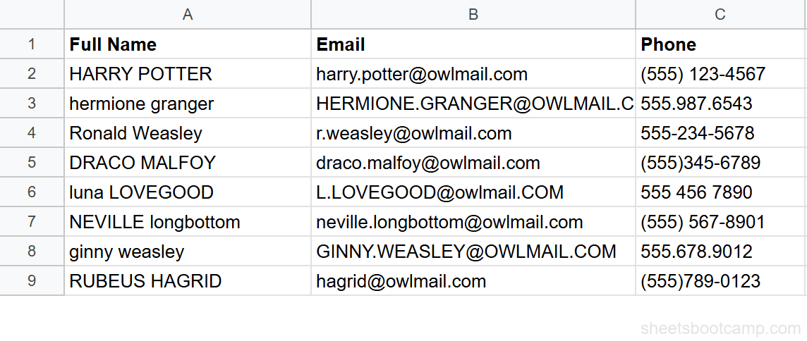
We’ll standardize the messy phone numbers in the contacts table.
1
Set up your data
The contacts spreadsheet has phone numbers in column C in 4 formats: "(555) 123-4567", "555.987.6543", "555-234-5678", and "(555)345-6789". The goal is to strip all formatting down to 10 digits.
2
Replace hyphens with spaces
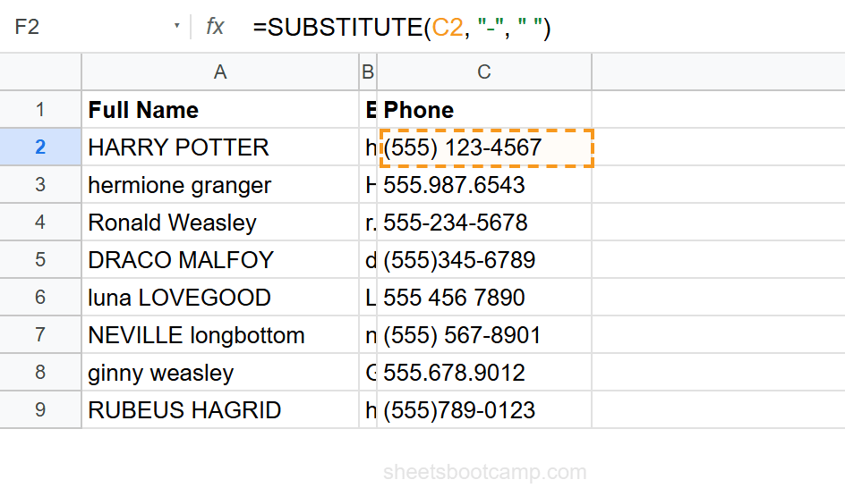
Select cell F2 and enter:
Formula
=SUBSTITUTE(C2, "-", " ") For "(555) 123-4567", this replaces the hyphen with a space, returning “(555) 123 4567”. The parentheses, spaces, and other characters are untouched. SUBSTITUTE only replaces what you tell it to.
3
Nest SUBSTITUTE to remove all formatting
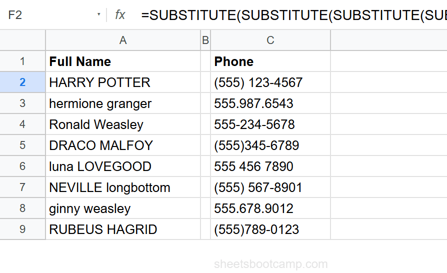
To strip every non-digit character, nest multiple SUBSTITUTE calls:
Formula
=SUBSTITUTE(SUBSTITUTE(SUBSTITUTE(SUBSTITUTE(SUBSTITUTE(C2,"(",""),")",""),"-",""),".","")," ","") Each layer removes one character type: parentheses, hyphens, periods, and spaces. The result is 5551234567. This works on every phone format in the data because it covers all the separators used.
4
Copy down and verify
Copy the formula down through row 9. Every phone number resolves to a clean 10-digit string regardless of the original format. For "555.987.6543", the period layer handles the dots. For "555 456 7890", the space layer removes the spaces.
Tip
For cleaner phone cleaning, consider REGEXREPLACE with a single pattern: =REGEXREPLACE(C2, ”[^0-9]”, ""). This removes all non-digit characters in one step instead of nesting five SUBSTITUTE calls.
The Instance Argument
By default, SUBSTITUTE replaces every occurrence. The fourth argument lets you target a specific one.
Formula
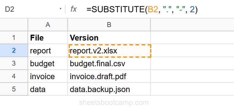
=SUBSTITUTE(B2, ".", "-", 2) For a filename like "report.v2.xlsx", this replaces only the second period with a hyphen, returning “report.v2-xlsx”. The first period stays.
| Instance | Result for "report.v2.xlsx" |
|---|---|
| Omitted | "report-v2-xlsx" (all replaced) |
| 1 | "report-v2.xlsx" (first only) |
| 2 | "report.v2-xlsx" (second only) |
This is useful when a string has multiple delimiters and you need to change one without affecting the others.
Nested SUBSTITUTE for Multiple Replacements
When you need to replace several different characters, nest SUBSTITUTE calls. Each layer handles one replacement, processing from the inside out.
Remove all currency formatting:
Formula
=SUBSTITUTE(SUBSTITUTE(SUBSTITUTE(A2, "$", ""), ",", ""), " ", "") For "$1,234.56", this removes the dollar sign and comma, returning "1234.56". Wrap in VALUE to convert to a number: =VALUE(SUBSTITUTE(SUBSTITUTE(SUBSTITUTE(A2, "$", ""), ",", ""), " ", "")).
Standardize separators:
Formula
=SUBSTITUTE(SUBSTITUTE(A2, "/", "-"), ".", "-") This converts both slashes and periods to hyphens. For "2026/05/15", it returns "2026-05-15". For "2026.05.15", same result.
SUBSTITUTE vs REPLACE
| Feature | SUBSTITUTE | REPLACE |
|---|---|---|
| Finds by | Text content | Position |
| Replaces | Matching text | Characters at position |
| Case-sensitive | Yes | N/A |
| Instance control | Yes (4th argument) | N/A |
| Use when | You know what to replace | You know where to replace |
SUBSTITUTE example: =SUBSTITUTE("hello world", "world", "sheets") returns "hello sheets".
REPLACE example: =REPLACE("hello world", 7, 5, "sheets") replaces 5 characters starting at position 7, returning "hello sheets".
SUBSTITUTE is the right choice when the text you want to change is consistent. REPLACE is better when the position is consistent but the content varies.
Practical Examples
Example 1: Clean Names with Extra Spaces
Multiple spaces between words cannot be fixed with TRIM alone if you want a specific separator. SUBSTITUTE with a targeted replacement handles it:
Formula
=SUBSTITUTE(TRIM(A2), " ", " ") Wait, TRIM already collapses multiple spaces to one. So TRIM alone handles this. Use SUBSTITUTE on top of TRIM when you need a different separator, like replacing spaces with underscores: =SUBSTITUTE(TRIM(A2), " ", "_") turns "SHERLOCK HOLMES" into "SHERLOCK_HOLMES".
Example 2: Build a URL Slug from a Title
Convert a title like "Monthly Sales Report" into a URL-friendly slug:
Formula
=LOWER(SUBSTITUTE(A2, " ", "-")) This replaces spaces with hyphens and converts to lowercase, returning “monthly-sales-report”.
Example 3: Mask a Phone Number
Show only the last 4 digits of a phone number:
Formula
=SUBSTITUTE(C2, LEFT(C2, LEN(C2) - 4), "***-***-") For "(555) 123-4567", this replaces everything except the last 4 characters with a mask, returning “--4567”.
Common Errors and How to Fix Them
No Replacement Happens
SUBSTITUTE is case-sensitive. If the search text does not match the case in the cell, nothing changes. =SUBSTITUTE("HELLO", "hello", "hi") returns "HELLO" unchanged. Convert to a common case first: =SUBSTITUTE(LOWER(A2), "hello", "hi").
Unexpected Double Replacements
If you replace “a” with “ab” and the original text is “aa”, the result is “abab”, not “aab”. SUBSTITUTE scans left to right and does not re-process replaced text. This is rarely an issue, but be aware of it when the replacement text contains the search text.
#N/A or #VALUE! Errors
SUBSTITUTE does not return these errors on its own. If you see errors, they come from another function in the formula chain. Check the input cell. If it contains an error, SUBSTITUTE passes it through.
Note
SUBSTITUTE returns the original text unchanged when the search text is not found. It does not error. This makes it safe to apply SUBSTITUTE broadly even when some cells do not contain the target character.
Tips and Best Practices
-
Use empty string "" to delete characters.
=SUBSTITUTE(A2, "-", "")is the standard pattern for removing a character entirely. -
Nest from the inside out. When nesting multiple SUBSTITUTE calls, the innermost one runs first. Put the most common replacement innermost for readability.
-
SUBSTITUTE preserves formulas. Unlike Find and Replace (Ctrl+H), SUBSTITUTE works inside formulas and does not modify the source cell. Use it in helper columns for clean data while keeping the original intact.
-
Use the instance argument for multi-delimiter strings. When a string has the same character used as different delimiters (like periods in filenames), the fourth argument targets exactly the one you want.
-
Consider REGEXREPLACE for pattern-based replacements. When you need to remove all non-digits, all non-letters, or any pattern-based replacement, one REGEXREPLACE call replaces multiple nested SUBSTITUTE calls.
Related Google Sheets Tutorials
- Text Functions in Google Sheets: Full guide to cleaning, extracting, and combining text
- FIND and SEARCH in Google Sheets: Locate text positions before replacing
- TRIM and CLEAN in Google Sheets: Remove extra spaces and invisible characters
- REGEXMATCH, REGEXEXTRACT, REGEXREPLACE: Pattern-based text matching and replacement
- LEFT, RIGHT, MID in Google Sheets: Extract specific characters by position
Frequently Asked Questions
What does the SUBSTITUTE function do in Google Sheets?
SUBSTITUTE replaces all occurrences of a specified text string with new text inside a formula. For example, =SUBSTITUTE(A2, "-", " ") replaces every hyphen with a space. Unlike Find and Replace (Ctrl+H), SUBSTITUTE works inside formulas and does not modify the original cell.
Is SUBSTITUTE case-sensitive in Google Sheets?
Yes. SUBSTITUTE is case-sensitive. =SUBSTITUTE("Hello", "hello", "Hi") returns "Hello" unchanged because "hello" does not match "Hello". To replace regardless of case, convert the text to one case first or use REGEXREPLACE with a case-insensitive flag.
How do I replace only the second occurrence with SUBSTITUTE?
Use the fourth argument (instance_num). =SUBSTITUTE(A2, ".", "-", 2) replaces only the second period with a hyphen. Instance 1 replaces only the first, instance 2 only the second, and so on. Omit this argument to replace all occurrences.
What is the difference between SUBSTITUTE and REPLACE in Google Sheets?
SUBSTITUTE finds and replaces specific text strings. REPLACE replaces characters at a specific position regardless of what those characters are. Use SUBSTITUTE when you know what text to replace. Use REPLACE when you know the position of the characters to replace.
Can I nest multiple SUBSTITUTE functions?
Yes. Wrap one SUBSTITUTE inside another to replace multiple different characters. =SUBSTITUTE(SUBSTITUTE(A2, "-", ""), ".", "") removes both hyphens and periods. Each SUBSTITUTE handles one replacement, and they process from the inside out.
You've googled this formula before. Probably more than once.
The Bootcamp is a real Google Sheet that grades every formula the moment you press Enter. 193 exercises across 9 modules, the 10% of Sheets that does 90% of the work. One payment of $29.
Get It for $29 Get the Bootcamp for $2930-day refund. Reply to any email and you get your money back.
Not ready to pay? Try Basic Training free →