
FIND is case-sensitive. =FIND(“holmes”, “SHERLOCK HOLMES”) returns a #VALUE! error because lowercase “holmes” does not match uppercase “HOLMES”. Use SEARCH when case does not matter.
beginner 6 min read
FIND and SEARCH Functions in Google Sheets
Use FIND and SEARCH in Google Sheets to locate text inside a cell. Learn the syntax, differences, wildcard support, and how to combine them with other functions.
SB
Sheets Bootcamp
March 11, 2026 · Updated May 14, 2026
Table of Contents
The FIND function in Google Sheets returns the position of a character or substring inside a text string. SEARCH does the same thing but ignores case and supports wildcards. The text functions guide covers the full set of text tools, and FIND and SEARCH are the foundation for dynamic text extraction when you combine them with LEFT, RIGHT, and MID.
This guide covers both functions, when to use each, and how to pair them with other formulas for real data tasks.
In This Guide
- FIND Syntax and Parameters
- SEARCH Syntax and Parameters
- FIND vs SEARCH: When to Use Each
- Locate Text Step-by-Step
- Practical Examples
- Wildcard Searches with SEARCH
- Common Errors and How to Fix Them
- Tips and Best Practices
- Related Google Sheets Tutorials
- Frequently Asked Questions
FIND Syntax and Parameters
FIND returns the position of a substring within a text string. It is case-sensitive.
Formula
=FIND(search_for, text_to_search, [starting_at]) | Argument | Description | Required |
|---|---|---|
| search_for | The text to find | Yes |
| text_to_search | The cell or string to search in | Yes |
| starting_at | Position to start searching from (default: 1) | No |
Example: =FIND("@", "sherlock.holmes@bakermail.com") returns 16. The @ symbol is the 16th character.
Important
SEARCH Syntax and Parameters
SEARCH returns the position of a substring within a text string. It is case-insensitive and supports wildcards.
Formula
=SEARCH(search_for, text_to_search, [starting_at]) | Argument | Description | Required |
|---|---|---|
| search_for | The text to find (supports ? and * wildcards) | Yes |
| text_to_search | The cell or string to search in | Yes |
| starting_at | Position to start searching from (default: 1) | No |
Example: =SEARCH("holmes", "SHERLOCK HOLMES") returns 12. SEARCH matches despite the case difference.
Wildcards in SEARCH:
?matches any single character*matches any sequence of characters
FIND vs SEARCH: When to Use Each
| Feature | FIND | SEARCH |
|---|---|---|
| Case-sensitive | Yes | No |
| Wildcards (? and *) | No | Yes |
| Performance | Same | Same |
| Starting position | Yes | Yes |
Use FIND when the case of the text matters, like distinguishing between product codes “ABC” and “abc”. Use SEARCH for everything else. Since most text lookups do not require case sensitivity, SEARCH is the more common choice.
Locate Text Step-by-Step
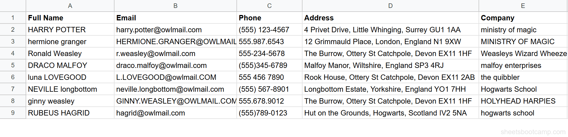
We’ll use the messy contacts table to locate characters in email addresses and names.
1
Open the contacts spreadsheet
The table has 8 contacts with emails in column B. Some emails are lowercase (sherlock.holmes@bakermail.com), some are uppercase (JOHN.WATSON@BAKERMAIL.COM), and some are mixed (M.MORSTAN@bakermail.COM).
2
Find the @ symbol position with FIND
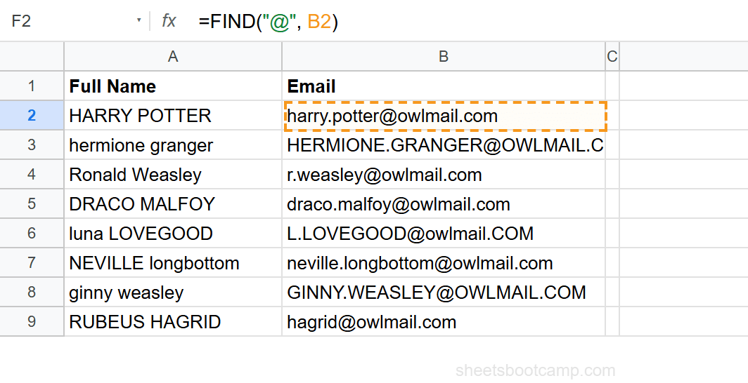
Select cell F2 and enter:
Formula
=FIND("@", B2) For "sherlock.holmes@bakermail.com", FIND returns 16. The @ symbol is at position 16. Copy down through row 9. Every email has an @ symbol, so FIND works on all rows.
3
Extract the username with LEFT and FIND
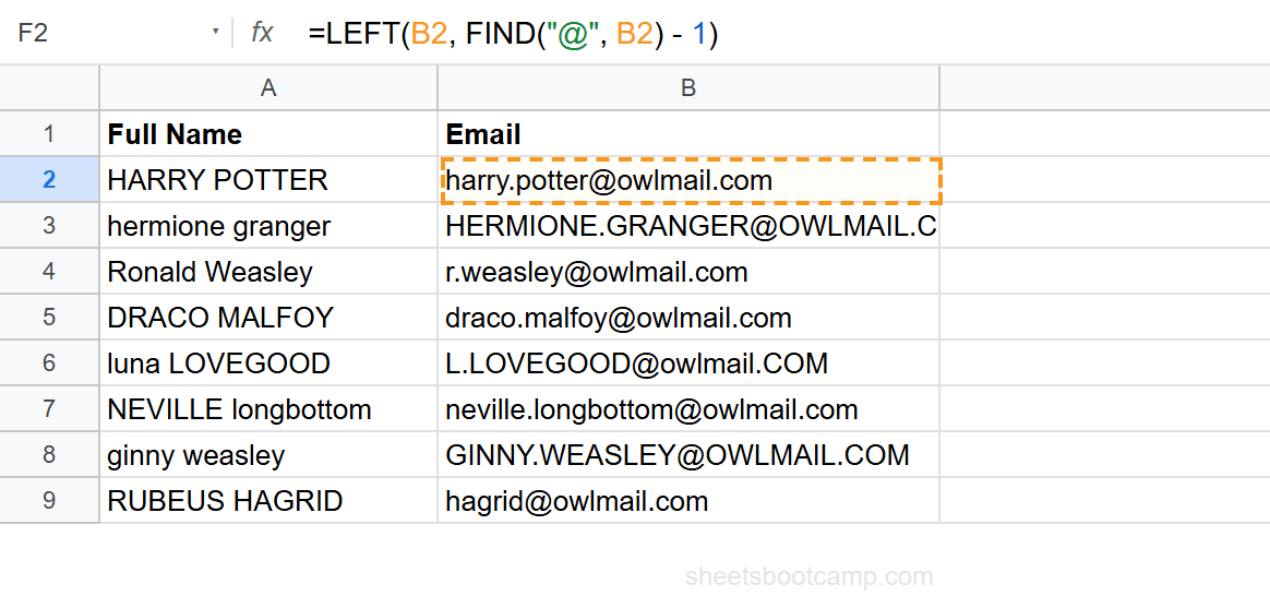
Select cell G2 and enter:
Formula
=LEFT(B2, FIND("@", B2) - 1) FIND returns 16. Subtracting 1 gives 15. LEFT returns the first 15 characters: sherlock.holmes. This dynamic extraction works regardless of username length.
4
Test SEARCH for case-insensitive matching
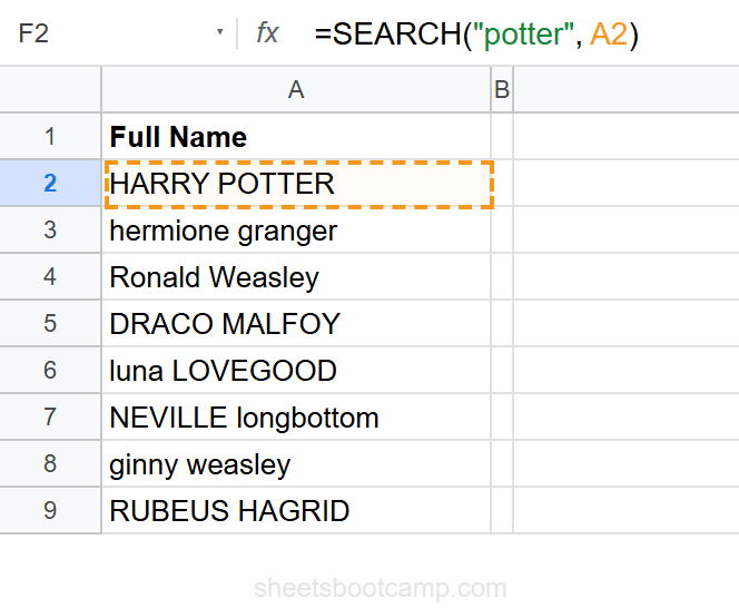
Select cell H2 and enter:
Formula
=SEARCH("holmes", A2) Cell A2 contains "SHERLOCK HOLMES" in all caps. SEARCH returns 12 because it ignores case and finds “HOLMES” starting at position 12 (after “SHERLOCK ”). FIND would return an error here because “holmes” does not match “HOLMES”.
Note
The position count includes every character, including spaces. In “SHERLOCK HOLMES”, the three spaces between the names count as positions 9, 10, and 11. HOLMES starts at position 12.
Practical Examples
Example 1: Check If a Cell Contains Text
To check if a cell contains a specific word, wrap SEARCH in ISNUMBER:
Formula
=ISNUMBER(SEARCH("holmes", A2)) SEARCH returns a number if it finds the text, or an error if it does not. ISNUMBER converts this to TRUE or FALSE. For "SHERLOCK HOLMES", this returns TRUE. For " Inspector Lestrade ", it returns FALSE.
Combine with IF to return a label: =IF(ISNUMBER(SEARCH("holmes", A2)), "Holmes family", "Other").
Example 2: Find the Second Occurrence
Use the starting_at argument to skip past the first match:
Formula
=FIND(".", B2, FIND(".", B2) + 1) The inner FIND locates the first period in the email. Adding 1 moves past it. The outer FIND searches from that new position. For "sherlock.holmes@bakermail.com", the first period is at position 9. The second period is at position 26 (in “bakermail.com”). This returns 26.
Example 3: Extract Domain from Email
Combine FIND with MID to get everything after the @ symbol:
Formula
=MID(B2, FIND("@", B2) + 1, LEN(B2)) FIND returns 16. Adding 1 starts MID at position 17. LEN provides a count larger than the remaining characters, so MID returns everything from position 17 to the end: bakermail.com.
Wildcard Searches with SEARCH
SEARCH supports two wildcards that FIND does not:
Question mark (?) matches one character:
Formula
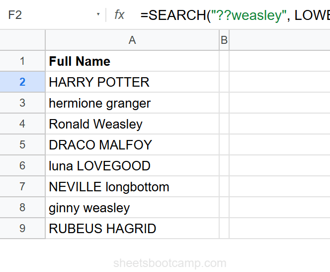
=SEARCH("??holmes", LOWER(TRIM(A2))) This finds any two characters followed by “holmes”. For "sherlock holmes" (after LOWER and TRIM), the "k " before “holmes” matches the two ? wildcards, and SEARCH returns 8.
Asterisk (*) matches any number of characters:
Formula
=SEARCH("h*r", A2) This finds text that starts with “h” and ends with “r” with any characters in between. For "SHERLOCK HOLMES", SEARCH matches “HER” (the first h through the next r) starting at position 2 and returns 2.
Tip
To search for an actual question mark or asterisk (not as wildcards), precede it with a tilde: =SEARCH(”~?”, A2) finds a literal question mark.
Common Errors and How to Fix Them
#VALUE! Error: Text Not Found
Both FIND and SEARCH return #VALUE! when the search text does not exist in the cell. Wrap in IFERROR to handle missing text: =IFERROR(FIND("@", A2), 0) returns 0 when there is no @ symbol.
#VALUE! Error: Case Mismatch (FIND Only)
FIND is case-sensitive. =FIND("abc", "ABC") returns #VALUE!. Switch to SEARCH if case does not matter, or convert the text first: =FIND("abc", LOWER(A2)).
#VALUE! Error: Starting Position Beyond Text Length
If starting_at is greater than the length of the text, both functions return #VALUE!. Check with LEN first: =IF(LEN(A2) >= 5, FIND("x", A2, 5), "Too short").
Tip
Always wrap FIND or SEARCH in IFERROR when the search text might not exist in every row. One missing match causes the entire column to show errors if you copy the formula down.
Tips and Best Practices
-
Default to SEARCH unless case matters. SEARCH handles both cases and supports wildcards. FIND is only needed when you must distinguish between uppercase and lowercase.
-
Combine with LEFT, MID, or RIGHT for extraction. FIND and SEARCH return position numbers, not the text itself. Use the position as an argument in LEFT, RIGHT, or MID to pull the actual text.
-
Use starting_at to find the Nth occurrence. Nest FIND calls to skip past earlier matches.
=FIND(",", A2, FIND(",", A2) + 1)finds the second comma. -
Wrap in ISNUMBER for TRUE/FALSE checks.
=ISNUMBER(SEARCH("text", A2))is the standard pattern for checking if a cell contains text. It returns TRUE or FALSE without errors. -
SUBSTITUTE is better for replacing text. FIND and SEARCH locate text. If you need to replace it, use SUBSTITUTE or the REGEX functions instead.
Related Google Sheets Tutorials
- Text Functions in Google Sheets: Full guide to cleaning, extracting, and combining text
- LEFT, RIGHT, MID in Google Sheets: Extract characters using positions from FIND or SEARCH
- SUBSTITUTE Function in Google Sheets: Replace text in formulas instead of locating it
- SPLIT Function in Google Sheets: Separate text at delimiters into columns
- IF Function in Google Sheets: Conditional logic with ISNUMBER and SEARCH
Frequently Asked Questions
What is the difference between FIND and SEARCH in Google Sheets?
FIND is case-sensitive and does not support wildcards. SEARCH is case-insensitive and supports wildcards (? for one character, * for any number). Use FIND when case matters and SEARCH when it does not.
How do I find the position of a character in a cell in Google Sheets?
Use =FIND(character, cell) or =SEARCH(character, cell). Both return the position number of the first occurrence. For example, =FIND("@", B2) returns the position of the @ symbol in an email address.
Can FIND or SEARCH return the position of the second occurrence?
Yes. Use the optional starting_at argument. =FIND(".", B2, FIND(".", B2) + 1) finds the second period by starting the search one position after the first period.
Why does FIND return an error when the text exists in the cell?
FIND is case-sensitive. If you search for "holmes" but the cell contains "HOLMES", FIND returns #VALUE! because the cases do not match. Use SEARCH instead for case-insensitive matching.
How do I check if a cell contains specific text in Google Sheets?
Wrap SEARCH in ISNUMBER: =ISNUMBER(SEARCH("text", A2)). This returns TRUE if the text exists anywhere in the cell, FALSE otherwise. SEARCH is case-insensitive, so it matches regardless of capitalization.
You've googled this formula before. Probably more than once.
The Bootcamp is a real Google Sheet that grades every formula the moment you press Enter. 193 exercises across 9 modules, the 10% of Sheets that does 90% of the work. One payment of $29.
Get It for $29 Get the Bootcamp for $2930-day refund. Reply to any email and you get your money back.
Not ready to pay? Try Basic Training free →