VLOOKUP with ARRAYFORMULA in Google Sheets
Learn how to use VLOOKUP with ARRAYFORMULA in Google Sheets to fill an entire column with one formula. Step-by-step examples and error handling.
Sheets Bootcamp
March 14, 2026 · Updated April 29, 2026
VLOOKUP works on one cell at a time. If you have 100 rows that need a lookup, you write the formula once and copy it down 99 times. Wrapping VLOOKUP in ARRAYFORMULA eliminates the copying. One formula in one cell fills the entire column.
This guide covers how to set up the ARRAYFORMULA wrapper, handle empty rows and errors, and when this approach works best.
In This Guide
- How ARRAYFORMULA Works with VLOOKUP
- Basic VLOOKUP ARRAYFORMULA
- Handling Empty Rows
- Handling Errors
- Step-by-Step: Price Lookup for Sales Data
- Open-Ended Ranges for Auto-Expanding Data
- Performance Considerations
- Tips and Best Practices
- Related Google Sheets Tutorials
- Frequently Asked Questions
How ARRAYFORMULA Works with VLOOKUP
A standard VLOOKUP takes a single search key and returns a single result:
=VLOOKUP(D2, Products!A2:D12, 4, FALSE)ARRAYFORMULA takes that single-cell formula and applies it to an entire range of search keys:
=ARRAYFORMULA(VLOOKUP(D2:D10, Products!A2:D12, 4, FALSE))The key change: D2 becomes D2:D10. ARRAYFORMULA tells Google Sheets to run the VLOOKUP for every cell in that range and return all results at once. The results spill down from the cell where you entered the formula.
The cells below the ARRAYFORMULA cell must be empty. If any cell in the spill range already has data, the formula returns a #REF! error.
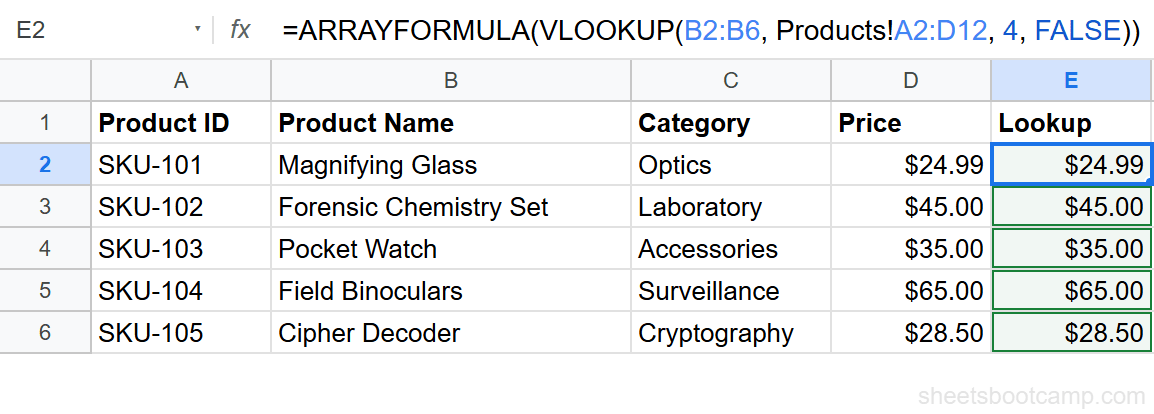
Basic VLOOKUP ARRAYFORMULA
Here is the basic pattern:
=ARRAYFORMULA(VLOOKUP(A2:A10, LookupTable, column_number, FALSE))| Component | Purpose |
|---|---|
ARRAYFORMULA(...) | Tells Google Sheets to process an array of values |
A2:A10 | The range of search keys (replaces a single cell) |
LookupTable | The range to search in (stays the same for all rows) |
column_number | Which column to return (stays the same for all rows) |
FALSE | Exact match (stays the same for all rows) |
Handling Empty Rows
The basic ARRAYFORMULA runs VLOOKUP on every cell in the range, including empty cells. Empty cells produce #N/A errors because VLOOKUP cannot find a blank value.
Wrap the VLOOKUP in IF to skip empty cells:
=ARRAYFORMULA(IF(A2:A10="", "", VLOOKUP(A2:A10, LookupTable, 2, FALSE)))The IF checks each cell. If the cell is empty, it returns an empty string. If the cell has a value, it runs the VLOOKUP.
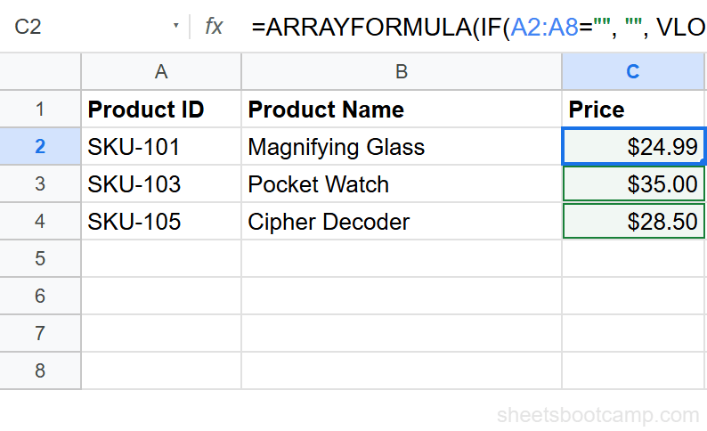
Without the IF wrapper, every empty row shows #N/A. On a sheet with 1,000 rows but only 50 with data, you get 950 error cells. Always include the IF check.
Handling Errors
Even with the IF wrapper for empty cells, some search keys may not exist in the lookup table. Add IFERROR inside the ARRAYFORMULA to catch those:
=ARRAYFORMULA(IF(A2:A10="", "", IFERROR(VLOOKUP(A2:A10, LookupTable, 2, FALSE), "Not found")))This formula handles three scenarios:
| Search key | Result |
|---|---|
| Valid value | Looked-up result |
| Empty cell | Empty string |
| Value not in table | ”Not found” |
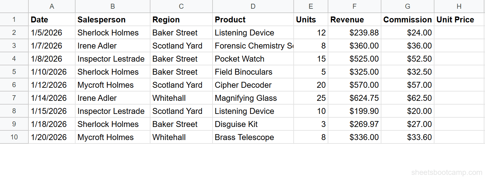
Step-by-Step: Price Lookup for Sales Data
We’ll add a product price column to the sales records by looking up each product in the inventory table.
Set up the source data and lookup column
The sales records have product names in column D. The product inventory has product names in column B and prices in column D. You want to add a “Unit Price” column to the sales records.
Write the ARRAYFORMULA with VLOOKUP
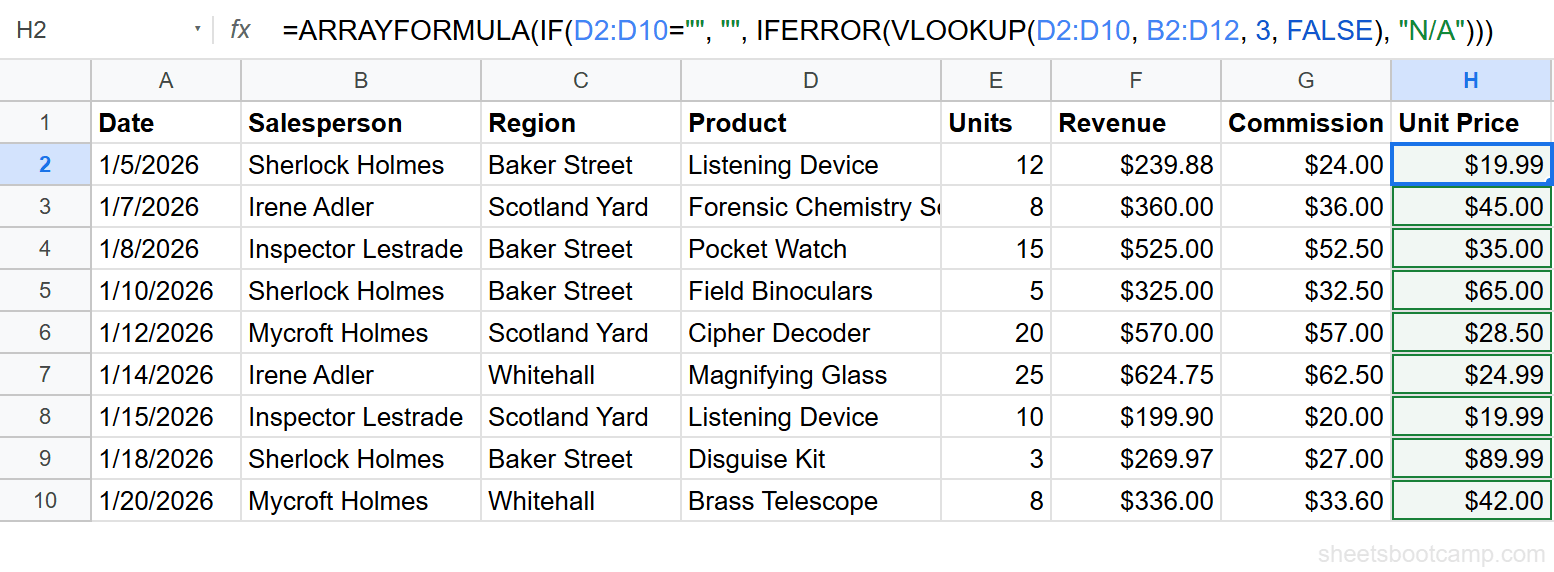
Enter the following formula in cell H2:
=ARRAYFORMULA(IF(D2:D10="", "", IFERROR(VLOOKUP(D2:D10, B2:D12, 3, FALSE), "N/A")))The formula searches column B of the product inventory for each product name from the sales records and returns the price from column D.
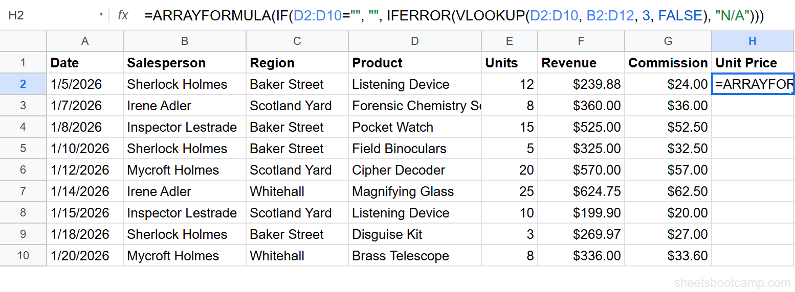
Review the auto-filled results
All 9 rows fill with the correct price. One formula, one cell, nine results.
You cannot edit or delete individual cells in the spill range. To modify results, edit the ARRAYFORMULA cell itself. To clear the results, delete the formula from the source cell.
Open-Ended Ranges for Auto-Expanding Data
Replace the fixed range D2:D10 with an open-ended range D2:D to handle new rows automatically:
=ARRAYFORMULA(IF(D2:D="", "", IFERROR(VLOOKUP(D2:D, B2:D12, 3, FALSE), "N/A")))When new sales are added in row 11, 12, etc., the formula automatically looks up their prices. The IF wrapper prevents blank rows from showing errors.
Open-ended ranges like D2:D extend to the bottom of the sheet (row 1,000 by default, or more if the sheet has been expanded). The IF check ensures VLOOKUP only runs on non-empty cells, so performance remains acceptable.
Performance Considerations
ARRAYFORMULA with VLOOKUP recalculates every row whenever any cell in the sheet changes. On small datasets this is instant. On large datasets, consider these trade-offs:
| Sheet size | ARRAYFORMULA VLOOKUP | Individual formulas |
|---|---|---|
| Under 1,000 rows | Fast, convenient | Works fine but more cells to manage |
| 1,000-10,000 rows | Noticeable lag on edits | Each cell recalculates independently (faster) |
| Over 10,000 rows | Can slow down the sheet | Better performance, or use XLOOKUP |
If your sheet becomes sluggish, consider switching from ARRAYFORMULA to individual VLOOKUP formulas, or using XLOOKUP which handles arrays natively and can be more efficient.
Tips and Best Practices
-
Always include the IF empty-cell check.
=ARRAYFORMULA(IF(range="", "", VLOOKUP(...)))prevents hundreds of#N/Aerrors on unused rows. -
Use IFERROR for invalid search keys. Some products may not exist in the lookup table. IFERROR catches these without breaking the entire array.
-
Use open-ended ranges for growing data.
D2:Dinstead ofD2:D10means you never need to update the formula when new rows are added. -
Do not put data below an ARRAYFORMULA. The spill range must be clear. If a cell below has data, the formula returns
#REF!. Leave the column dedicated to the ARRAYFORMULA. -
Absolute references for the lookup range. Use
$B$2:$D$12or a named range for the lookup table. This does not affect ARRAYFORMULA behavior but makes the formula clearer.
Related Google Sheets Tutorials
- VLOOKUP in Google Sheets - Complete guide to VLOOKUP syntax and features
- ARRAYFORMULA in Google Sheets - Full guide to ARRAYFORMULA for any function
- VLOOKUP with IF - Add conditions to your lookups
- VLOOKUP for Beginners - Start here if you are new to VLOOKUP
- INDEX MATCH with ARRAYFORMULA - The INDEX MATCH version of array lookups
Frequently Asked Questions
Can I use VLOOKUP with ARRAYFORMULA in Google Sheets?
Yes. Wrap your VLOOKUP in ARRAYFORMULA and use a range as the search key instead of a single cell: =ARRAYFORMULA(VLOOKUP(A2:A10, data, 2, FALSE)). The formula spills results down the entire column.
Why does VLOOKUP ARRAYFORMULA show #N/A for empty rows?
ARRAYFORMULA runs VLOOKUP for every cell in the range, including empty ones. Empty cells return #N/A because VLOOKUP cannot find a blank value. Wrap in IF to skip blank cells: =ARRAYFORMULA(IF(A2:A="", "", VLOOKUP(A2:A, data, 2, FALSE))).
Is ARRAYFORMULA VLOOKUP slower than copying formulas down?
On small datasets (under 1,000 rows), performance is similar. On large datasets (10,000+ rows), ARRAYFORMULA can be slower because it recalculates every row when any cell changes. For very large sheets, individual formulas or XLOOKUP may perform better.
How do I handle errors in VLOOKUP ARRAYFORMULA?
Wrap in IFERROR inside the ARRAYFORMULA: =ARRAYFORMULA(IFERROR(VLOOKUP(A2:A, data, 2, FALSE), "Not found")). IFERROR catches errors for each row individually.
Can I use an open-ended range with VLOOKUP ARRAYFORMULA?
Yes. Use A2:A instead of A2:A10 as the search key. The formula automatically extends to new rows. Combine with IF to skip empty cells and avoid unnecessary #N/A errors.