INDEX MATCH with ARRAYFORMULA in Google Sheets

INDEX MATCH normally looks up one value at a time. Wrapping it in ARRAYFORMULA applies the lookup to every row in a column, so one formula in one cell replaces dozens or hundreds of copied formulas. This guide covers the exact pattern, common pitfalls, and when to use open-ended ranges for growing data.

In This Guide

• Why Use ARRAYFORMULA with INDEX MATCH?
• The Formula Pattern
• Step-by-Step Setup
• Handle Blank Rows
• Open-Ended Ranges for Growing Data
• Common Errors
• Tips
• Related Google Sheets Tutorials
• Frequently Asked Questions

Why Use ARRAYFORMULA with INDEX MATCH?

When you have a column of lookup values (like a list of Product IDs), the standard approach is to write an INDEX MATCH formula in the first row and copy it down. This works, but it creates a separate formula in every cell.

Problems with copying formulas down:

• Hundreds of individual formulas slow down recalculation
• New rows require manually copying the formula to each one
• Editing the formula means updating every cell, not just one

ARRAYFORMULA solves these by putting one formula in one cell. The formula processes the entire column and fills results into the rows below automatically.

The Formula Pattern

The ARRAYFORMULA version of INDEX MATCH wraps the entire formula and passes a column range instead of a single cell as the search key:

=ARRAYFORMULA(IF(search_column="", "", INDEX(return_range, MATCH(search_column, lookup_range, 0))))

The IF wrapper handles blank rows. Without it, empty cells in the search column produce #N/A errors.

Step-by-Step Setup

We’ll look up prices from the product inventory for a list of Product IDs.

Sample Data

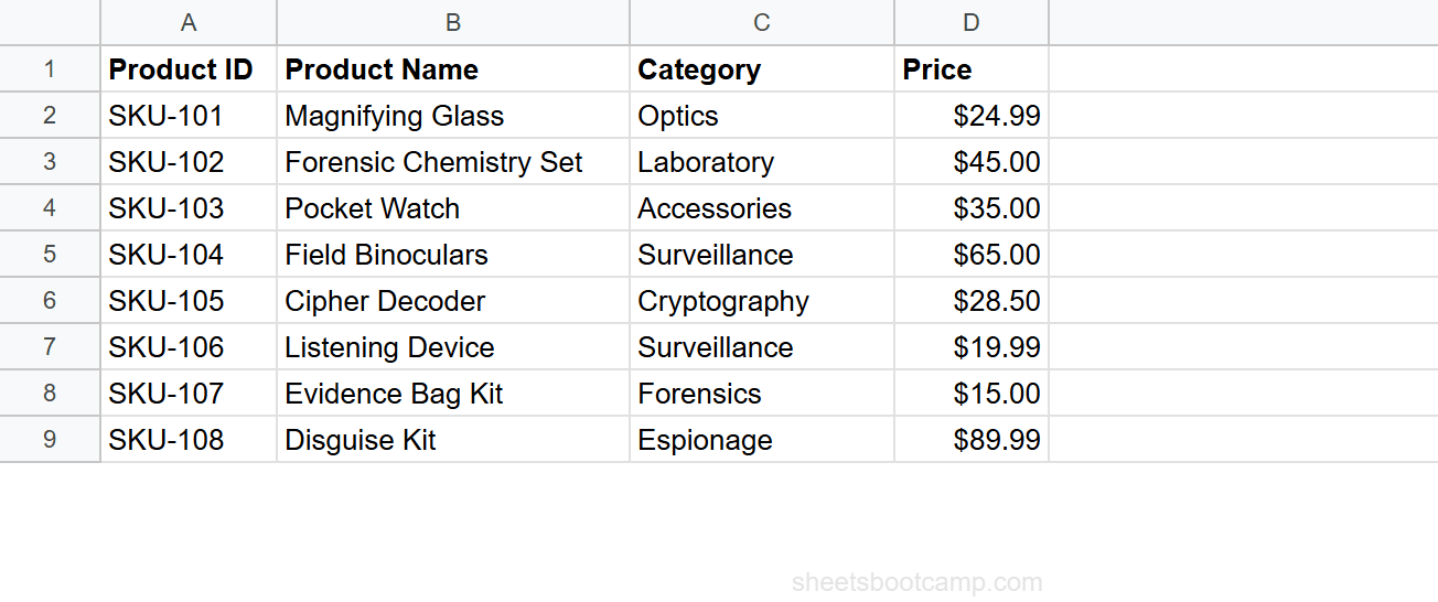
The product inventory has Product IDs in column A and Prices in column D (8 products, rows 2 through 9). A separate list of Product IDs sits in column H (4 IDs in H2:H5).

The inventory table runs from A1:F9. The lookup list in H2:H5 contains four Product IDs: SKU-103, SKU-106, SKU-101, and SKU-108. You want to return the price for each one in column I.

Start with a standard INDEX MATCH formula in I2:

=INDEX(D2:D9, MATCH(H2, A2:A9, 0))

This returns $35.00 — the price for SKU-103. But it only works for one row. You would need to copy this formula to I3, I4, and I5 for the other Product IDs.

Replace the single cell reference H2 with the column range H2:H5, and wrap everything in ARRAYFORMULA with an IF check for blanks:

=ARRAYFORMULA(IF(H2:H5="", "", INDEX(D2:D9, MATCH(H2:H5, A2:A9, 0))))

Enter this formula in I2 only. It returns prices for all four Product IDs at once:

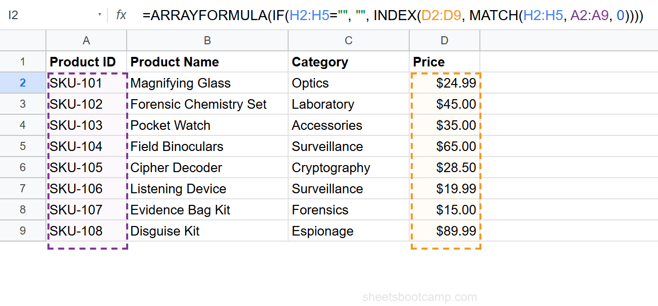
One formula, four results. Cells I3:I5 show results but contain no formula of their own — they are filled by the ARRAYFORMULA in I2.

Handle Blank Rows

Without the IF wrapper, blank cells in the search column cause MATCH to look for an empty string, which produces #N/A errors.

The IF check suppresses this:

=ARRAYFORMULA(IF(H2:H5="", "", INDEX(D2:D9, MATCH(H2:H5, A2:A9, 0))))

When H3 is empty, the formula returns an empty string for that row instead of an error. All other rows still return their lookup results.

Open-Ended Ranges for Growing Data

If new Product IDs get added to column H regularly, use an open-ended range:

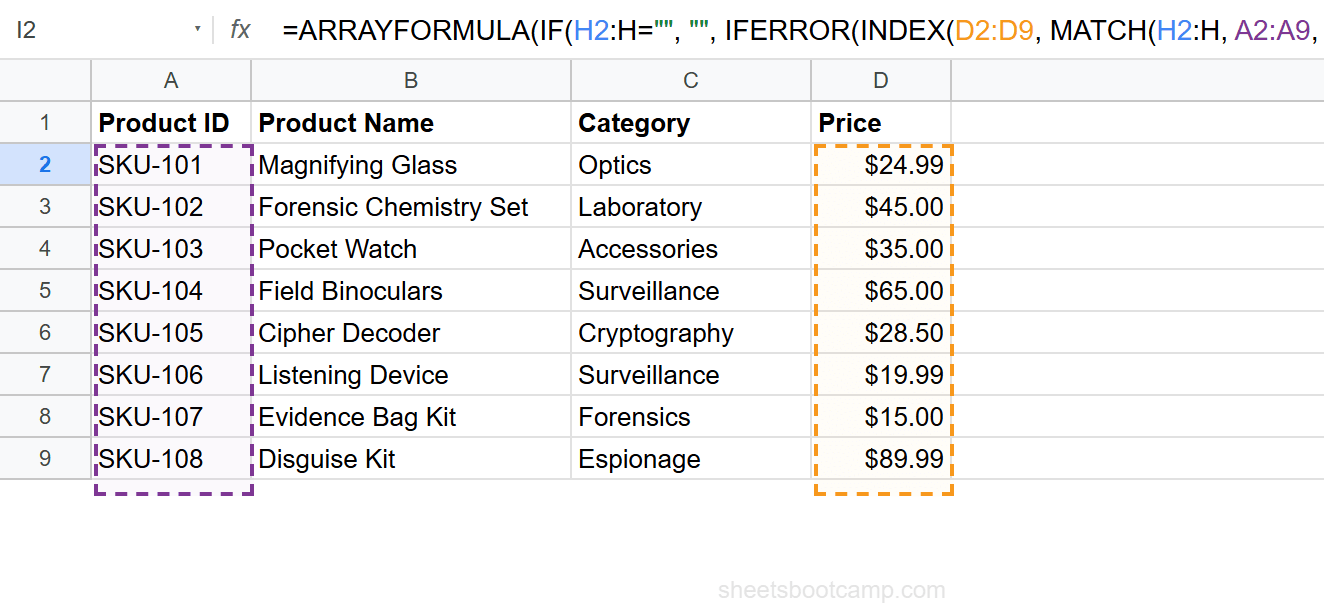
=ARRAYFORMULA(IF(H2:H="", "", IFERROR(INDEX(D2:D9, MATCH(H2:H, A2:A9, 0)), "Not found")))

H2:H (no end row) means “H2 to the bottom of the sheet.” New IDs added in H6, H7, or beyond are included automatically.

Common Errors

#REF! — Cells below are not empty

ARRAYFORMULA needs empty cells below the formula cell to spill results into. If I3 contains a value or formula, the ARRAYFORMULA in I2 returns #REF!.

Fix: Clear all cells in the output column below the formula cell.

#N/A — Lookup value not found

A Product ID in column H does not exist in the inventory. MATCH cannot find it and returns #N/A.

Fix: Wrap in IFERROR: IFERROR(INDEX(..., MATCH(...)), "Not found").

Only one result returned

If the ARRAYFORMULA returns only the first result instead of filling all rows, check that the search key argument is a range (H2:H5), not a single cell (H2).

Fix: Change MATCH(H2, ...) to MATCH(H2:H5, ...) inside the ARRAYFORMULA.

Slow performance

ARRAYFORMULA with open-ended ranges on large sheets (10,000+ rows) can be slow because Google Sheets evaluates the formula for every row.

Fix: Use a bounded range (H2:H500) instead of H2:H. Or split the data across multiple sheets.

Tips

1. Always include the IF blank check. IF(H2:H="", "", ...) prevents #N/A errors on empty rows. This is the most common issue with ARRAYFORMULA INDEX MATCH.

2. Use IFERROR for missing values. Not every lookup value may exist in the source data. IFERROR handles this gracefully without breaking the array.

3. Keep the lookup table fixed with absolute references. The return range (D2:D9) and lookup range (A2:A9) should not shift. Since ARRAYFORMULA processes from one cell, absolute references ($D$2:$D$9) are good practice.

4. This pattern also works with VLOOKUP. See VLOOKUP with ARRAYFORMULA for the VLOOKUP equivalent. The structure is the same: wrap in ARRAYFORMULA, pass a column range, add an IF blank check.

5. For returning multiple matching rows, use FILTER. ARRAYFORMULA with INDEX MATCH returns one result per search key. If a single search key has multiple matches, see INDEX MATCH to return multiple results.

Related Google Sheets Tutorials

• INDEX MATCH: The Complete Guide — Full syntax, left lookups, and the combined formula pattern
• INDEX MATCH for Beginners — Step-by-step tutorial for your first formula
• ARRAYFORMULA: Complete Guide — Apply any formula to an entire column at once
• VLOOKUP with ARRAYFORMULA — The VLOOKUP version of this pattern
• INDEX MATCH to Return Multiple Results — Return all matching rows, not just the first

Frequently Asked Questions

Can I use INDEX MATCH with ARRAYFORMULA?

Yes. Wrap the formula in ARRAYFORMULA and pass a column range as the search key: =ARRAYFORMULA(INDEX(return_range, MATCH(search_column, lookup_range, 0))). The formula returns results for every row in the search column.

Why does my ARRAYFORMULA INDEX MATCH return only one result?

INDEX with a single-column range ignores the array from MATCH and returns only the first result. Use ARRAYFORMULA(IF(ISNA(…))) or switch to a multi-row INDEX range trick. The simplest fix is to wrap the MATCH result in a conditional check.

Is ARRAYFORMULA with INDEX MATCH faster than copying formulas down?

A single ARRAYFORMULA is generally faster than hundreds of individual formulas because Google Sheets processes it as one calculation instead of many. It also keeps your sheet cleaner with one formula instead of one per row.

What happens when new rows are added?

If your ARRAYFORMULA references open-ended ranges like A2:A (no end row), new rows are included automatically. Use open-ended ranges for data that grows over time.

Can I use ARRAYFORMULA with INDEX MATCH MATCH?

ARRAYFORMULA works with the row MATCH but not easily with the column MATCH in a two-way lookup. For two-way lookups across multiple rows, write individual INDEX MATCH MATCH formulas instead.