VLOOKUP with Wildcards in Google Sheets
Learn how to use VLOOKUP with wildcards in Google Sheets for partial text matching. Use asterisk and question mark wildcards with real examples.
Sheets Bootcamp
March 16, 2026 · Updated April 23, 2026
VLOOKUP with wildcards in Google Sheets lets you search for partial text instead of requiring an exact match. When your VLOOKUP search key is only part of the value in your data, wildcards fill in the rest.
This guide covers both wildcard characters (asterisk and question mark), how to combine them with cell references, and the edge cases that trip people up.
In This Guide
- How Wildcards Work in VLOOKUP
- Asterisk Wildcard: Match Any Characters
- Question Mark Wildcard: Match One Character
- Using Wildcards with Cell References
- Searching for Literal Wildcards
- Common Errors and How to Fix Them
- Tips and Best Practices
- Related Google Sheets Tutorials
- Frequently Asked Questions
How Wildcards Work in VLOOKUP
Google Sheets VLOOKUP supports two wildcard characters when the last argument is FALSE (exact match mode):
| Wildcard | Matches | Example |
|---|---|---|
* (asterisk) | Any number of characters (including zero) | "*Chemistry Set" matches “Forensic Chemistry Set” |
? (question mark) | Exactly one character | "SKU-10?" matches “SKU-101” through “SKU-109” |
You can combine multiple wildcards in a single search key. "*Quill*" matches anything containing “Quill” anywhere in the text.
Wildcards only work with text values. If the first column of your range contains numbers or dates, wildcards have no effect.
Asterisk Wildcard: Match Any Characters
The asterisk (*) is the most common wildcard. It matches any sequence of characters, including an empty string.
Starts with
To find a product name that starts with specific text:
=VLOOKUP("Nimbus*", B2:D6, 3, FALSE)This matches “Magnifying Glass” and returns $24.99 from column D.
Ends with
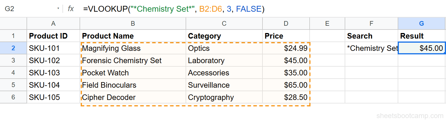
To find a product name that ends with specific text:
=VLOOKUP("*Chemistry Set", B2:D6, 3, FALSE)This matches “Forensic Chemistry Set” and returns $45.00.
Contains
To find a product name that contains specific text anywhere:
=VLOOKUP("*Stirring*", B2:D6, 3, FALSE)This also matches “Forensic Chemistry Set” and returns $45.00.
Question Mark Wildcard: Match One Character
The question mark (?) matches exactly one character. It is useful when you know the pattern but one character varies.
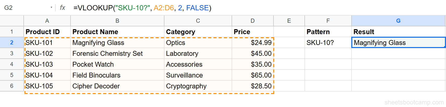
=VLOOKUP("SKU-10?", A2:D6, 2, FALSE)This matches “SKU-101” (the first row where column A has a value matching the pattern) and returns “Magnifying Glass” from column B.
To match two unknown characters, use two question marks:
=VLOOKUP("SKU-1??", A2:D6, 2, FALSE)This also matches “SKU-101” since ?? covers the “01” portion.
The question mark is strict about character count. "SKU-10?" matches “SKU-101” but not “SKU-1001” because the question mark replaces only one character.
Using Wildcards with Cell References
Hardcoding the search term works for one-off lookups, but in practice you want the wildcard to reference a cell. Concatenate the asterisk with the cell reference using the & operator.
Step-by-Step Example
We’ll use the product inventory with 5 items. The goal: look up the price by entering part of a product name.
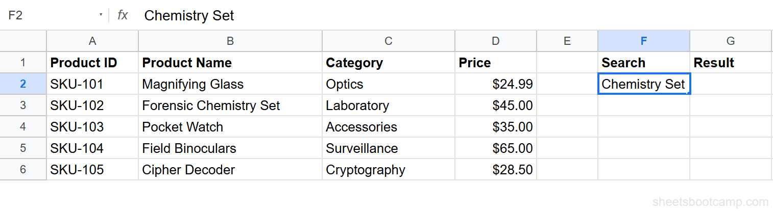
Set up your data with a partial search term
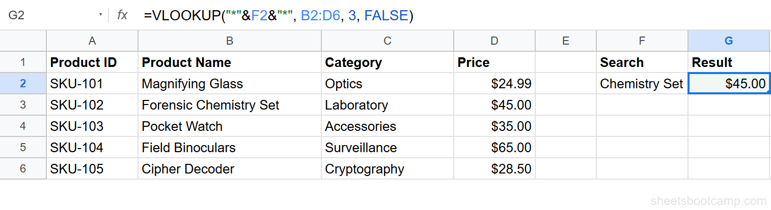
Enter “Chemistry Set” in cell F2. This is the partial name you want to search for.
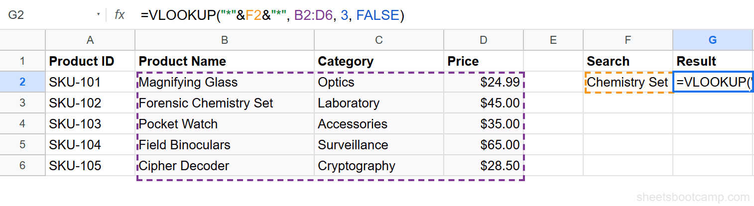
Write the VLOOKUP formula with asterisk wildcards
Enter the following formula in cell G2:
=VLOOKUP("*"&F2&"*", B2:D6, 3, FALSE)The "*"&F2&"*" portion builds the search key *Chemistry Set* by wrapping the cell value in asterisks. VLOOKUP then searches column B for any product name containing “Chemistry Set.”
Review the result
The formula returns $45.00 because “Forensic Chemistry Set” contains the word “Chemistry Set.” Change F2 to “Nimbus” and the result updates to $24.99.
Wildcard matching is not case-sensitive. Searching for “chemistry set” matches “Forensic Chemistry Set” the same way “Chemistry Set” does.
Searching for Literal Wildcards
If your data actually contains an asterisk or question mark character, prefix the wildcard with a tilde (~) to tell VLOOKUP to treat it as a literal character.
=VLOOKUP("Price~*", A2:B10, 2, FALSE)This searches for the literal text “Price*” instead of treating * as a wildcard.
| Escape Sequence | Searches For |
|---|---|
~* | Literal asterisk character |
~? | Literal question mark character |
~~ | Literal tilde character |
Common Errors and How to Fix Them
#N/A Error
The wildcard pattern did not match any value in the first column. Check for:
- Wrong column in range. If your product names are in column B, the range must start at B, not A. VLOOKUP searches the first column of the range.
- Numbers instead of text. Wildcards only match text. If the first column contains numbers, convert them to text or use a different approach.
- Extra spaces. Trailing spaces prevent matches. Wrap your wildcard formula in TRIM or use
"*"&TRIM(F2)&"*"to clean the input.
Unexpected Result (Wrong Row Returned)
VLOOKUP returns the first match from top to bottom. If multiple rows match the wildcard pattern, you get the first one. Sort your data or use a more specific pattern to control which row matches.
Wrap wildcard VLOOKUP in IFERROR to return a custom message when no match exists: =IFERROR(VLOOKUP("*"&F2&"*", B2:D6, 3, FALSE), "No match found").
Tips and Best Practices
-
Use
"*"&cell&"*"for “contains” searches. This is the most common wildcard pattern. It matches the cell value anywhere in the target text. -
Be specific to avoid false matches.
"*ear*"matches “Listening Device” but also “Year-End Report.” Add more characters to your pattern to narrow results. -
Combine wildcards.
"S*Chemistry Set"matches “Forensic Chemistry Set” but not “Iron Chemistry Set” because it requires the text to start with “S.” -
Consider FILTER for multiple results. VLOOKUP returns only the first match. If you need every row that contains the search term, use
=FILTER(A2:D6, REGEXMATCH(B2:B6, "(?i)Chemistry Set"))instead. -
VLOOKUP wildcards work with INDEX MATCH too. The MATCH function supports the same wildcard characters when its third argument is 0 (exact match).
Related Google Sheets Tutorials
- VLOOKUP in Google Sheets - Complete guide covering syntax, examples, and all VLOOKUP features
- VLOOKUP for Beginners - Start here if you are new to VLOOKUP
- Fix VLOOKUP Errors - Troubleshoot #N/A, #REF!, and #VALUE! errors
- INDEX MATCH in Google Sheets - A more flexible alternative for complex lookups
- VLOOKUP with Multiple Criteria - Look up values using two or more conditions
Frequently Asked Questions
Does VLOOKUP support wildcards in Google Sheets?
Yes. VLOOKUP supports two wildcards when using exact match (FALSE): the asterisk (*) matches any number of characters, and the question mark (?) matches exactly one character.
How do I search for a partial match with VLOOKUP?
Use an asterisk wildcard in your search key. For example, =VLOOKUP("*Chemistry Set*", A2:D6, 2, FALSE) finds any value containing the word “Chemistry Set” in the first column of the range.
Can I use wildcards with cell references in VLOOKUP?
Yes. Concatenate the asterisk with the cell reference: =VLOOKUP("*"&A1&"*", B2:D10, 2, FALSE). This searches for any value containing the text in A1.
How do I search for a literal asterisk or question mark with VLOOKUP?
Place a tilde (~) before the wildcard character. Use ~* to search for a literal asterisk and ~? to search for a literal question mark.
What happens if a wildcard VLOOKUP matches multiple rows?
VLOOKUP returns the first match it finds, scanning from top to bottom. If you need all matches, use FILTER instead.