Does Google Sheets have icon sets like Excel?

No. Google Sheets does not have a built-in icon set feature for conditional formatting. You can replicate the effect by using IF or IFS formulas with CHAR() or emoji characters to generate icons in a helper column, then applying conditional formatting to color them by status.

How do I add emoji icons based on cell values in Google Sheets?

Create a helper column with an IF or IFS formula that returns different emojis based on a condition. For example, =IF(D2="Complete", CHAR(9989), CHAR(10060)) returns a green checkmark for Complete and a red X for other values. You can also paste emoji characters directly into the formula.

Can I change emoji colors with conditional formatting?

Conditional formatting changes cell background and text color, but most emojis are rendered as images by the operating system and ignore text color. CHAR()-based symbols like checkmarks and X marks do respond to text color rules. Use CHAR(10004) for a checkmark and CHAR(10008) for an X if you need color control.

How do I create a traffic light system in Google Sheets?

Use an IFS formula to return colored circle emojis based on thresholds. For example, =IFS(F2>=80, CHAR(128994), F2>=50, CHAR(128993), TRUE, CHAR(128308)) returns a green circle for 80 or above, yellow for 50 to 79, and red below 50.

What is the difference between CHAR() symbols and emoji in Google Sheets?

CHAR() returns Unicode characters that render as plain text. They respond to font color and conditional formatting text color rules. Emojis are graphical characters rendered by the operating system. They appear in color regardless of text formatting. Use CHAR() when you need color control and emojis when you want universally recognizable icons.

Conditional Formatting Icons in Google Sheets

Conditional formatting icons in Google Sheets let you add visual status indicators to your data using formulas and formatting rules. Unlike Excel, Sheets does not have a built-in icon set feature, but you can build the same effect with conditional formatting and a few helper columns. The result: a color-coded dashboard where status is visible at a glance.

We’ll cover how to create icon columns with IF and CHAR(), color them with conditional formatting rules, and build traffic-light emoji indicators using IFS formulas.

How Icon Sets Work in Google Sheets

Excel has a built-in icon set feature that drops arrows, traffic lights, or checkmarks into cells based on value thresholds. Google Sheets does not offer this. Instead, you build it yourself in two parts:

A formula column that returns a symbol (via CHAR() or direct emoji) based on cell values
Conditional formatting rules that color the symbol based on the same values

The formula generates the icon. The formatting controls the color. Together, they replicate what Excel does with one click, except you get more control over which icons appear and how they look.

Sample Data

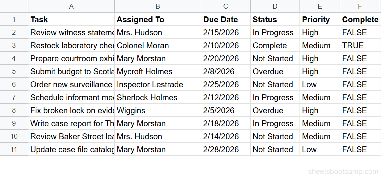
We’ll use a task tracker with 10 tasks. Columns A through F contain Task, Assigned To, Due Date, Status, Priority, and Complete.

	A	B	C	D	E	F
1	Task	Assigned To	Due Date	Status	Priority	Complete
2	Review witness statements	Mrs. Hudson	2/15/2026	In Progress	High	FALSE
3	Restock laboratory chemicals	Colonel Moran	2/10/2026	Complete	Medium	TRUE
4	Prepare courtroom exhibits	Mary Morstan	2/20/2026	Not Started	High	FALSE
5	Submit budget to Scotland Yard	Mycroft Holmes	2/8/2026	Overdue	High	FALSE
6	Order new surveillance equipment	Inspector Lestrade	2/25/2026	Not Started	Low	FALSE
7	Schedule informant meetings	Sherlock Holmes	2/12/2026	In Progress	Medium	FALSE
8	Fix broken lock on evidence room	Wiggins	2/5/2026	Overdue	High	FALSE
9	Write case report for The Strand	Mary Morstan	2/18/2026	In Progress	Medium	FALSE
10	Review Baker Street leads	Mrs. Hudson	2/14/2026	Not Started	Medium	FALSE
11	Update case file catalog	Mary Morstan	2/28/2026	Not Started	Low	FALSE

Step-by-Step: Build a Status Icon Column

Add a helper column with an IFS formula

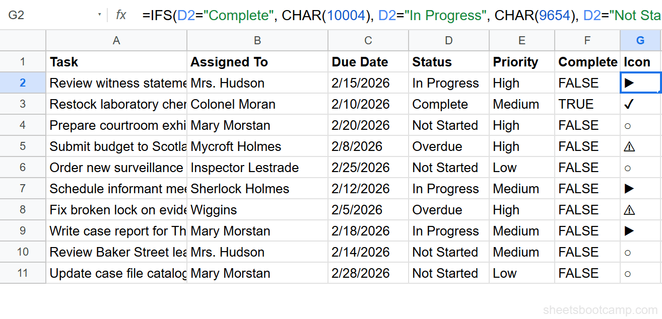
In cell G1, enter the header Icon. In G2, enter this formula:

Formula

=IFS(D2="Complete", CHAR(10004), D2="In Progress", CHAR(9654), D2="Not Started", CHAR(9675), TRUE, CHAR(9888))

This returns a different symbol for each status:

Status	CHAR Code	Symbol	Meaning
Complete	10004	✔	Checkmark
In Progress	9654	▶	Play/arrow
Not Started	9675	○	Open circle
Overdue	9888	⚠	Warning sign

Copy G2 down through G11. Every row now shows a symbol based on its Status value.

Important

CHAR() symbols render as plain text characters. They inherit the cell’s font color, which is why conditional formatting can change their color. Emojis are graphical and ignore text color settings.

Apply conditional formatting to color the icons

Select G2:G11. Go to Format > Conditional formatting. Create four rules, each using Custom formula is:

Rule 1, Complete (green):

Formula

=$D2="Complete"

Set text color to green (#34a853).

Rule 2, Overdue (red):

Formula

=$D2="Overdue"

Set text color to red (#ea4335).

Rule 3, In Progress (amber):

Formula

=$D2="In Progress"

Set text color to dark yellow (#f59e0b).

Rule 4, Not Started (gray):

Formula

=$D2="Not Started"

Set text color to gray (#9ca3af).

The $D2 reference locks to column D so the rule checks the Status column for every row in the icon column. For more on this technique, see formatting based on another cell.

Optional: Add a priority indicator column

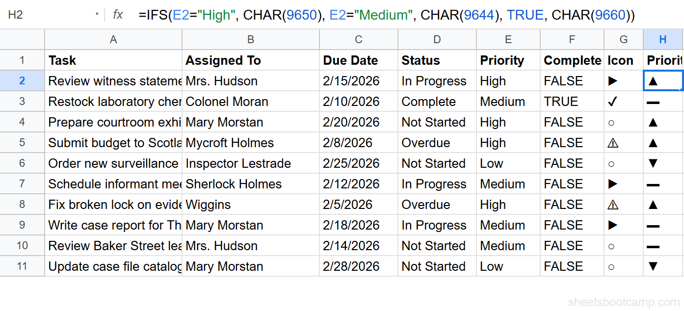
In column H, add a second icon column for Priority. In H2:

Formula

=IFS(E2="High", CHAR(9650), E2="Medium", CHAR(9644), TRUE, CHAR(9660))

Priority	CHAR Code	Symbol
High	9650	▲
Medium	9644	▬
Low	9660	▼

Apply conditional formatting rules to H2:H11: red text for High (=$E2="High"), amber for Medium, and blue for Low.

Review the visual dashboard

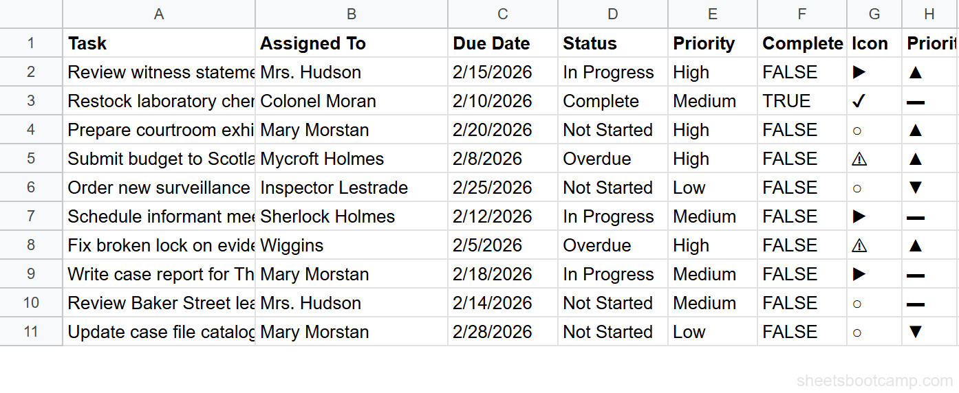
Your task tracker now has two icon columns. Each row displays its status and priority at a glance. Colonel Moran’s completed task shows a green checkmark and an amber dash. Mycroft Holmes’s overdue budget submission shows a red warning sign and a red up-arrow.

Traffic Light Emojis with IFS

If you want colored circles without conditional formatting, emoji characters handle both shape and color in one step. Unicode includes colored circle emojis that render consistently across platforms.

In a helper column, enter:

Formula

=IFS(F2=TRUE, CHAR(128994), D2="In Progress", CHAR(128993), D2="Overdue", CHAR(128308), TRUE, CHAR(11093))

Condition	CHAR Code	Color
Complete (TRUE)	128994	Green
In Progress	128993	Yellow
Overdue	128308	Red
Not Started	11093	White

This approach checks the Complete column (F) first. If F2=TRUE, the task gets a green circle. Otherwise, the formula checks the Status column for In Progress, Overdue, or defaults to a white circle for Not Started.

Note

Emoji rendering varies by device and operating system. What appears as a green filled circle on Windows may look slightly different on macOS or Android. CHAR()-based symbols are more consistent across platforms because they render as text glyphs.

Combining Approaches

You can use both techniques in the same sheet. CHAR() symbols with conditional formatting give you full control over colors and font size. Emoji circles work as a self-contained traffic light with no formatting rules needed. Pick whichever fits your use case, or use one column for status and the other for priority.

CHAR() vs. Emoji: When to Use Each

Feature	CHAR() Symbols	Emoji Characters
Color control	Yes, responds to text color and conditional formatting	No, emojis are graphical and ignore text color
Platform consistency	High, renders as a text glyph in the cell’s font	Varies, depends on OS and browser
Available icons	Checkmarks, arrows, circles, triangles, warning signs	Hundreds of options including faces, objects, flags
Readability at small sizes	Good, scales with font size	Can be hard to distinguish at small font sizes
Best for	Status dashboards where color coding matters	Quick visual tags where built-in color is enough

Use CHAR() when you need custom formula conditional formatting to control the icon’s appearance. Use emojis when the icon’s built-in color already communicates the meaning.

Tips and Best Practices

Keep icon columns narrow. Set column width to 30-40 pixels and center-align the cells. The icons stand out more when they are not surrounded by whitespace.
Use data validation for the Status column. A dropdown list prevents typos that break your IFS formula. If someone enters “complete” instead of “Complete,” the formula falls through to the default case. See checkbox data validation for another way to track completion.
Freeze the icon columns next to the data. If your sheet scrolls horizontally, freeze the status icon column so it stays visible. Go to View > Freeze and select the appropriate column count.
Test CHAR codes before committing. Enter =CHAR(10004) in an empty cell to preview the symbol. Not all Unicode code points render in Google Sheets. Stick to common symbols in the 9000-10000 and 128000-129000 ranges.

Tip

You can type emojis directly into a formula with the emoji keyboard. On Windows, press Win + . to open it. On macOS, press Ctrl + Cmd + Space. This saves you from looking up CHAR codes for every emoji.

Conditional Formatting: Complete Guide: all rule types, color scales, and managing multiple formatting rules
Custom Formula Conditional Formatting: write your own formatting rules using any Google Sheets function
Format Based on Another Cell: apply formatting to one column based on values in a different column
Data Validation Checkboxes: add TRUE/FALSE checkboxes for task completion tracking

Conditional Formatting Icons in Google Sheets

In This Guide