Fix INDEX MATCH Errors in Google Sheets

INDEX MATCH errors in Google Sheets fall into a few predictable categories. The #N/A error means the value was not found, #NUM! means the ranges are different sizes, #REF! means a referenced range was deleted, and #VALUE! means a structural problem in the formula. This guide covers each error type, shows the exact cause, and walks through the fix.

In This Guide

• Debugging Strategy
• #N/A Error, Value Not Found
• #NUM! Error, Range Mismatch
• #REF! Error, Deleted Range
• #VALUE! Error, Formula Structure Problem
• Wrong Value (No Error)
• 0 Instead of a Value
• Hiding Errors with IFERROR
• Tips
• Related Google Sheets Tutorials
• Frequently Asked Questions

Debugging Strategy

Before fixing a specific error, isolate which function is causing it. INDEX MATCH combines two functions, so the error could come from either one.

The error message tells you the category:

• #N/A: MATCH did not find the search key, or the MATCH range is more than one column wide
• #NUM!: The MATCH position exceeds the INDEX range
• #REF!: A range the formula pointed at was deleted
• #VALUE!: The match_type argument is not a number

Pull the MATCH function out and test it on its own:

If MATCH returns a number, the issue is in the INDEX part. If MATCH returns an error, focus on the search key and lookup range.

Use =TYPE() to check whether values are text or numbers. If the search key is a number (1) but the lookup column stores text (“1”), MATCH will not find a match.

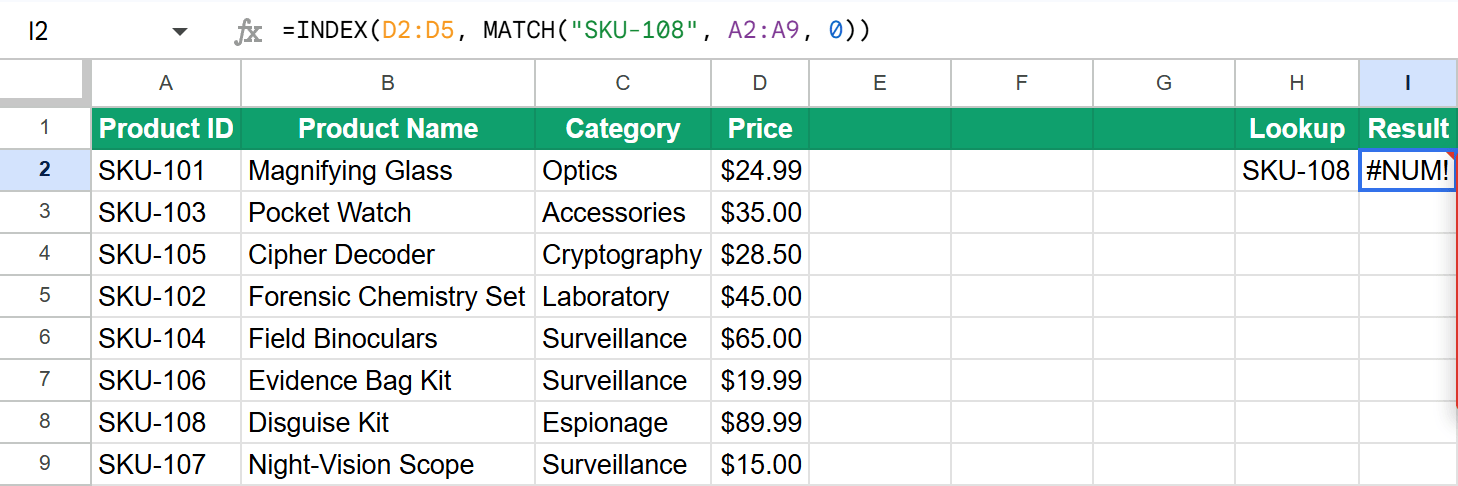
Count the rows in both ranges. If MATCH searches A2:A9 (8 rows) and INDEX references D2:D5 (4 rows), a match at position 5 or higher causes #NUM!.

#N/A Error: Value Not Found

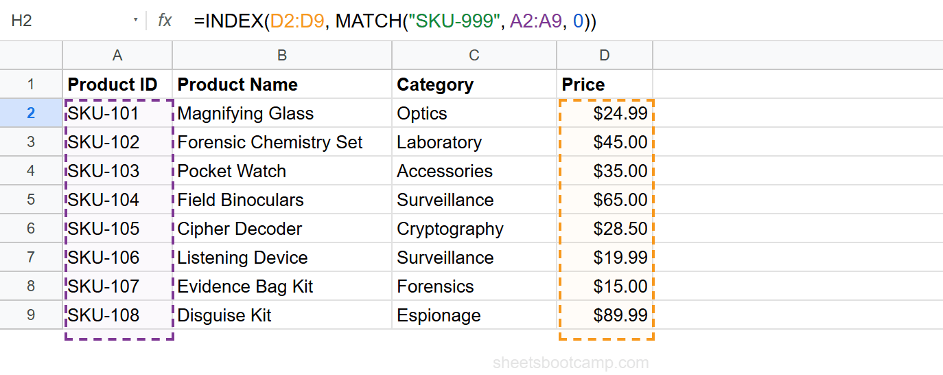
The #N/A error means MATCH searched the lookup range and could not find the search key. This is the most common INDEX MATCH error.

Cause 1: Typo or misspelling

The search key does not match any value in the lookup range. “Remebrall” (typo) does not match “Pocket Watch”.

Fix: Check the spelling of the search key against the actual data in the lookup column.

Cause 2: Extra spaces

The lookup value has trailing or leading spaces that are invisible but prevent matching. “SKU-103 ” (with a trailing space) does not match “SKU-103”.

Fix: Clean the data with TRIM: =INDEX(D2:D9, MATCH(TRIM(H2), A2:A9, 0)).

Cause 3: Mismatched data types

The search key is a number but the lookup column contains text (or vice versa). Cell A2 displays “103” but is stored as text, while the search key 103 is a number. They look identical but MATCH treats them as different values.

Fix: Use =TYPE(A2) and =TYPE(H2) to check. Type 1 = number, Type 2 = text. Convert with VALUE() or TEXT() to match types.

Cause 4: Missing 0 in MATCH (approximate match on unsorted data)

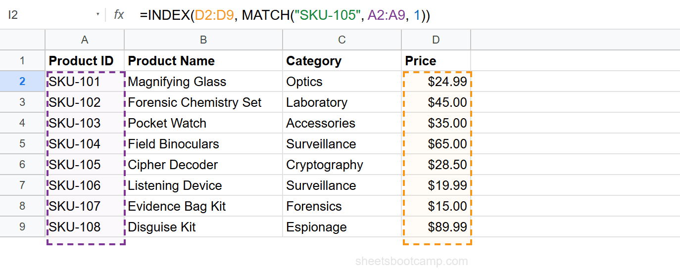
MATCH defaults to match_type 1 (approximate match) if you omit the third argument. On unsorted data, approximate matching returns the wrong position or #N/A.

Fix: Always include 0 as the third argument: MATCH(H2, A2:A9, 0).

Cause 5: Multi-column range in MATCH

MATCH works on a single column or a single row. Hand it a 2D range and it returns #N/A, not #VALUE!, even when the search key is visibly inside the range. =MATCH("SKU-103", A2:B9, 0) returns #N/A while =MATCH("SKU-103", A2:A9, 0) returns 3.

Fix: Use a single column: MATCH(H2, A2:A9, 0).

#NUM! Error: Range Mismatch

The #NUM! error means the position from MATCH exceeds the number of rows in the INDEX range.

Cause: INDEX range has fewer rows than MATCH range

MATCH searches A2:A9 (8 rows) and finds the value at position 7. INDEX references D2:D5 (4 rows). Position 7 does not exist in a 4-row range, so INDEX returns #NUM!.

Fix: Make both ranges the same size. If MATCH uses A2:A9, INDEX should use D2:D9:

#REF! Error: Deleted Range

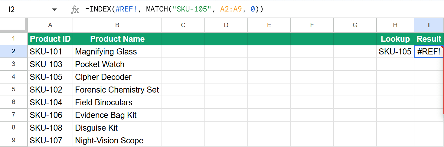
The #REF! error means a range the formula pointed at no longer exists, usually because someone deleted the column or the rows it referenced.

Cause: The referenced column or rows were deleted

Google Sheets rewrites the reference inside the formula itself. After column C is deleted, =INDEX(C2:C9, MATCH("SKU-105", A2:A9, 0)) becomes =INDEX(#REF!, MATCH("SKU-105", A2:A9, 0)).

Fix: Point the formula at the data’s new location. Nothing is wrong with the logic, the data moved out from under it. This is the most common INDEX MATCH failure in shared spreadsheets, and it is why named ranges are worth the setup time.

#VALUE! Error: Formula Structure Problem

The #VALUE! error means something is wrong with how the formula is constructed, not with the data.

Cause 1: Text instead of number for match_type

The third argument in MATCH must be a number. =MATCH("SKU-103", A2:A9, "x") returns #VALUE!.

Fix: Use 0 for exact match, not a text string.

Cause 2: Missing or extra argument

A misplaced comma or missing argument breaks the formula structure.

Fix: Check the formula for correct syntax: =INDEX(range, MATCH(key, range, 0)).

Wrong Value (No Error)

The formula returns a value, but it is from the wrong row. This is harder to catch because there is no error message.

Cause 1: Missing 0 in MATCH (approximate match)

Without the 0 third argument, MATCH uses approximate matching. On unsorted data, this returns whichever position the binary search algorithm lands on, which is unpredictable.

Fix: Add 0: MATCH(H2, A2:A9, 0).

Cause 2: Ranges start at different rows

MATCH searches A2:A9 and finds the value at position 3. INDEX references D5:D12 (starting at row 5 instead of row 2). Position 3 in D5:D12 is D7, but the correct value is in D4.

Fix: Start both ranges at the same row. Use A2:A9 and D2:D9.

Cause 3: Duplicate values in the lookup column

The lookup column has two identical entries. MATCH returns the first one. If you expected the second, the result is from the wrong row.

Fix: Use INDEX MATCH with multiple criteria to narrow the search. Or use the FILTER function to return all matching rows.

0 Instead of a Value

The formula returns 0 instead of the expected value. There is no error, but the result looks wrong.

Cause: The matched cell is empty

INDEX returns 0 when it references an empty cell. The lookup worked correctly and found the right position, but the return cell has no content. Google Sheets displays empty cells as 0 in formula results.

Fix: Check the return column at the matched position. If the cell is intentionally empty, wrap in an IF check:

Or use IFERROR combined with a check:

Hiding Errors with IFERROR

After fixing the root cause, wrap the formula in IFERROR to handle edge cases:

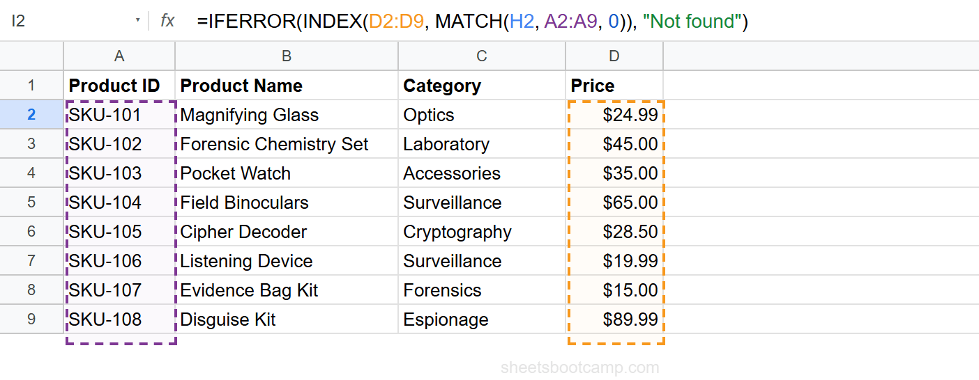
This returns “Not found” instead of any error. Use it for user-facing sheets where #N/A would be confusing.

Tips

1. Always test MATCH by itself first. =MATCH(H2, A2:A9, 0) should return a number. If it returns an error, focus on the MATCH arguments.

2. Always use 0 for exact match. Omitting the third argument in MATCH is the root cause of most INDEX MATCH problems. Make 0 a habit.

3. Use TYPE() to debug data type mismatches. =TYPE(A2) returns 1 for numbers and 2 for text. If the lookup column and search key have different types, MATCH will not find a match.

4. Check for invisible characters. Extra spaces, line breaks, and non-breaking spaces prevent matching. Use =LEN(A2) to check string length, if “SKU-103” shows length 8 instead of 7, there is an invisible character.

5. Validate range sizes. Count the rows in both ranges. They must match. A quick check: =ROWS(A2:A9) and =ROWS(D2:D9) should return the same number.

Related Google Sheets Tutorials

• INDEX MATCH: The Complete Guide: Full syntax, examples, and advanced patterns
• INDEX MATCH for Beginners: Step-by-step tutorial for your first formula
• INDEX MATCH with Multiple Criteria: Handle duplicate values with additional conditions
• Fix VLOOKUP Errors: Troubleshoot #N/A, #REF!, and #VALUE! in VLOOKUP
• IFERROR Function: Hide errors gracefully in any formula