Case-Sensitive VLOOKUP in Google Sheets

A case-sensitive VLOOKUP in Google Sheets requires a workaround because VLOOKUP ignores letter case by default. If your data contains values like “SKU-101” and “sku-101,” VLOOKUP treats them as identical and returns the first match it finds.

This guide shows you how to build a case-sensitive lookup using INDEX, MATCH, and EXACT. You will get a formula that distinguishes uppercase from lowercase, with step-by-step instructions and error fixes.

In This Guide

• Why VLOOKUP Ignores Case
• The Fix: INDEX + MATCH + EXACT
• Step-by-Step: Case-Sensitive Lookup
• Examples
• Common Errors and How to Fix Them
• Tips and Best Practices
• Related Google Sheets Tutorials
• Frequently Asked Questions

Why VLOOKUP Ignores Case

VLOOKUP in Google Sheets is case-insensitive by design. When you search for “sku-101,” it matches “SKU-101,” “Sku-101,” or any other capitalization variant. Google Sheets does not offer a built-in argument to change this behavior.

This creates a problem when your data has entries that differ only by case. Consider a product inventory where “SKU-101” and “sku-101” refer to different items. A standard VLOOKUP returns the first match from top to bottom, regardless of capitalization.

This formula returns “Magnifying Glass” (the first row with any case variation of “sku-101”) even if you intended to match the lowercase version on a different row.

The Fix: INDEX + MATCH + EXACT

The solution combines three functions:

• EXACT(text1, text2) compares two strings with case sensitivity. It returns TRUE only when every character matches, including uppercase and lowercase letters.
• MATCH(search_key, range, type) finds the position of a value in a range. When paired with EXACT, it locates the row where the case-sensitive match occurs.
• INDEX(range, row) returns the value at a specific position in a range.

The combined formula:

Here is how each piece works:

Step-by-Step: Case-Sensitive Lookup

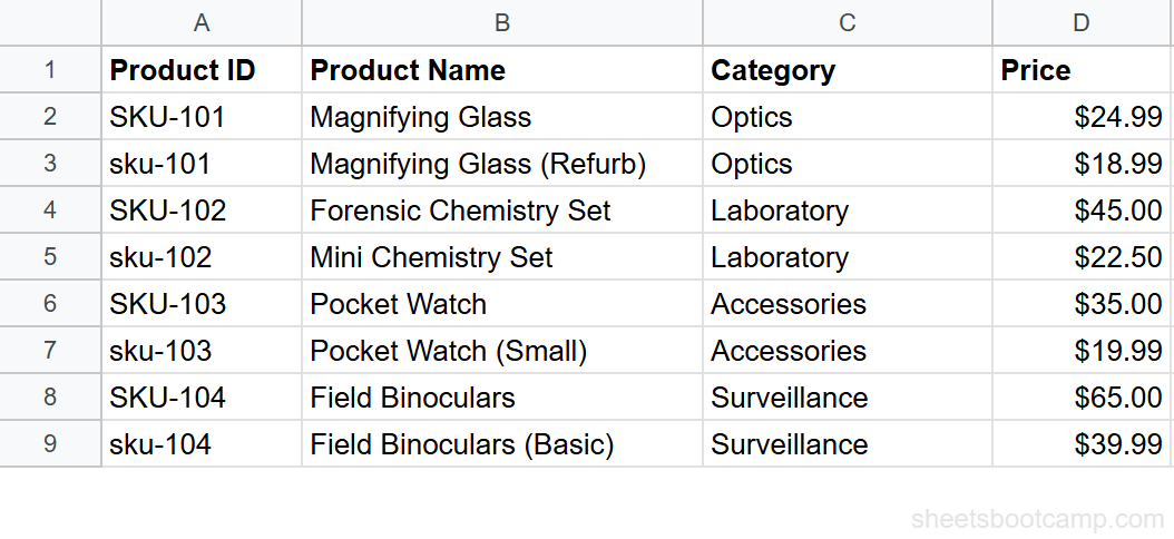
We will use the product inventory data. Imagine the sheet has both “SKU-101” and “sku-101” as Product IDs pointing to different items. The goal: look up the Category for “sku-101” specifically, not its uppercase counterpart.

Your data is in columns A through C. Column A has Product IDs, column B has Product Names, and column C has Categories. Enter the lookup value “sku-101” in cell F2.

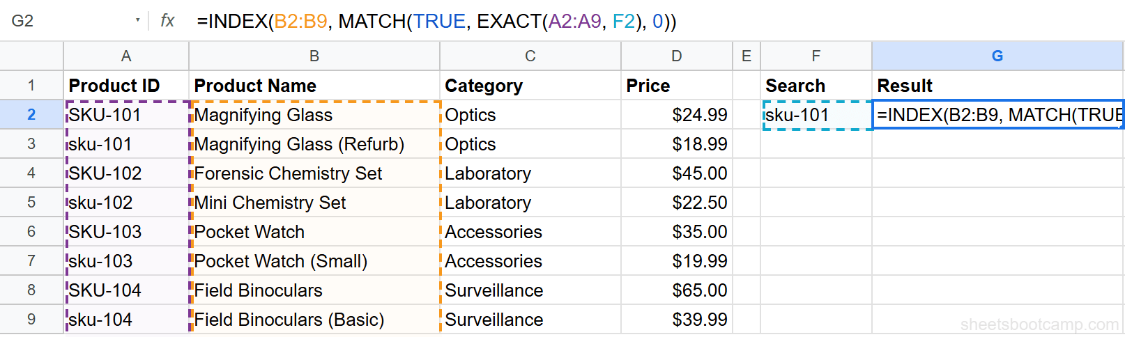
Select cell G2 and enter:

EXACT checks each Product ID in A2:A12 against the value in F2. Because F2 contains “sku-101” in lowercase, EXACT returns TRUE only for the row where column A also has “sku-101” in lowercase. MATCH finds that row position, and INDEX returns the Category from column C.

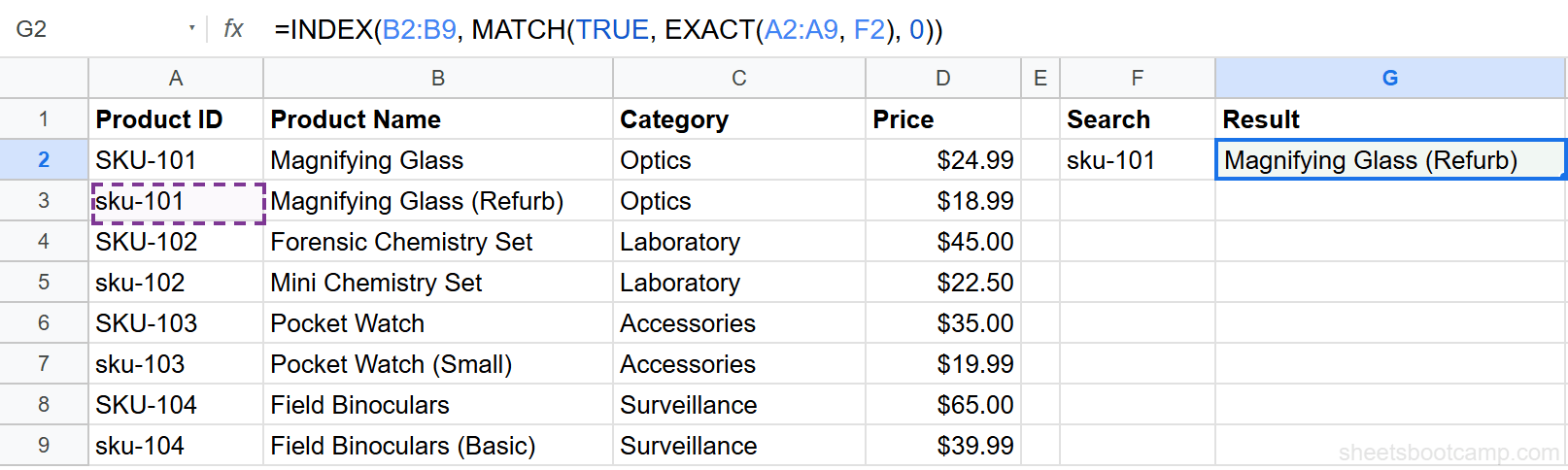
The formula returns the Category for the lowercase “sku-101” row. If you change F2 to “SKU-101” (uppercase), the result updates to show the Category for the uppercase row instead. This confirms the lookup is case-sensitive.

Examples

Example 1: Case-Sensitive Lookup Without ARRAYFORMULA

In some legacy guides, you will see the formula entered without ARRAYFORMULA and confirmed with Ctrl+Shift+Enter instead:

Press Ctrl+Shift+Enter after typing this formula. Google Sheets wraps it in curly braces {} to indicate it is processing as an array. The result is identical. However, using ARRAYFORMULA is the recommended approach because it works without a special keyboard shortcut.

Example 2: Case-Sensitive Price Lookup

To return the Price for a specific case-sensitive Product ID:

This returns $89.99, the price for “SKU-108” (Disguise Kit). If the sheet had a row with “sku-108” pointing to a different item, this formula would skip it and match only the uppercase version.

Common Errors and How to Fix Them

#N/A Error

The lookup value does not match any cell in the range when compared with exact case. This happens when:

• The capitalization is wrong. Double-check every character. “Sku-101” does not match “SKU-101” or “sku-101.”
• Extra spaces exist. A trailing space makes “SKU-101 ” different from “SKU-101.” Use =TRIM(F2) inside the formula: =INDEX(C2:C12, MATCH(TRUE, ARRAYFORMULA(EXACT(A2:A12, TRIM(F2))), 0)).
• The lookup range is wrong. Verify that A2:A12 covers all rows with data.

#VALUE! Error

This appears when the return range and lookup range have different sizes. Make sure both ranges have the same number of rows. If the lookup range is A2:A12 (11 rows), the return range must also be 11 rows, such as C2:C12.

Tips and Best Practices

1. Always use ARRAYFORMULA. It is more reliable than Ctrl+Shift+Enter and makes the formula self-documenting. Anyone reading it can see the array evaluation is intentional.

2. EXACT is strict about every character. Leading spaces, trailing spaces, and non-breaking spaces all cause mismatches. Clean your data with TRIM before running case-sensitive lookups.

3. Combine with data validation. If your Product IDs follow a specific case pattern (all uppercase, for example), use data validation to enforce it at entry time. Prevention beats troubleshooting.

4. Use named ranges for readability. Replace A2:A12 with a named range like ProductIDs. The formula becomes =INDEX(Categories, MATCH(TRUE, ARRAYFORMULA(EXACT(ProductIDs, F2)), 0)), which is easier to read and maintain.

5. Consider INDEX MATCH for all lookups. Once you are comfortable with this pattern, INDEX MATCH handles case sensitivity, left-side lookups, and multiple criteria. It covers gaps that VLOOKUP cannot.

Related Google Sheets Tutorials

• VLOOKUP in Google Sheets - Complete guide to VLOOKUP syntax, examples, and features
• Fix VLOOKUP Errors - Troubleshoot #N/A, #REF!, and #VALUE! errors in VLOOKUP formulas
• INDEX MATCH in Google Sheets - A flexible lookup method that handles case sensitivity and more
• VLOOKUP with ARRAYFORMULA - Apply VLOOKUP across multiple rows automatically