
To hide rows in Google Sheets, right-click the row numbers and choose Hide row, or press Ctrl+Alt+9. To unhide them, click the small arrow that appears on the row numbers next to the hidden rows, or press Ctrl+Shift+9. Columns work the same way with Ctrl+Alt+0 and Ctrl+Shift+0.
beginner 3 min read
How to Hide and Unhide Rows and Columns in Google Sheets
Hide and unhide rows or columns in Google Sheets with a right-click or a shortcut, group rows you can collapse, and find hidden rows. Includes Ctrl+Alt+9.
SB
Sheets Bootcamp
September 30, 2026
Table of Contents
Quick Answer
Hiding rows and columns is the quickest way to tidy a sheet without deleting anything. Helper columns, old months, and working calculations can all disappear from view and come back with one click. This page covers hiding and unhiding with the mouse and the keyboard, plus grouping, which is often the better choice.
How to Hide Rows
1
Select the rows
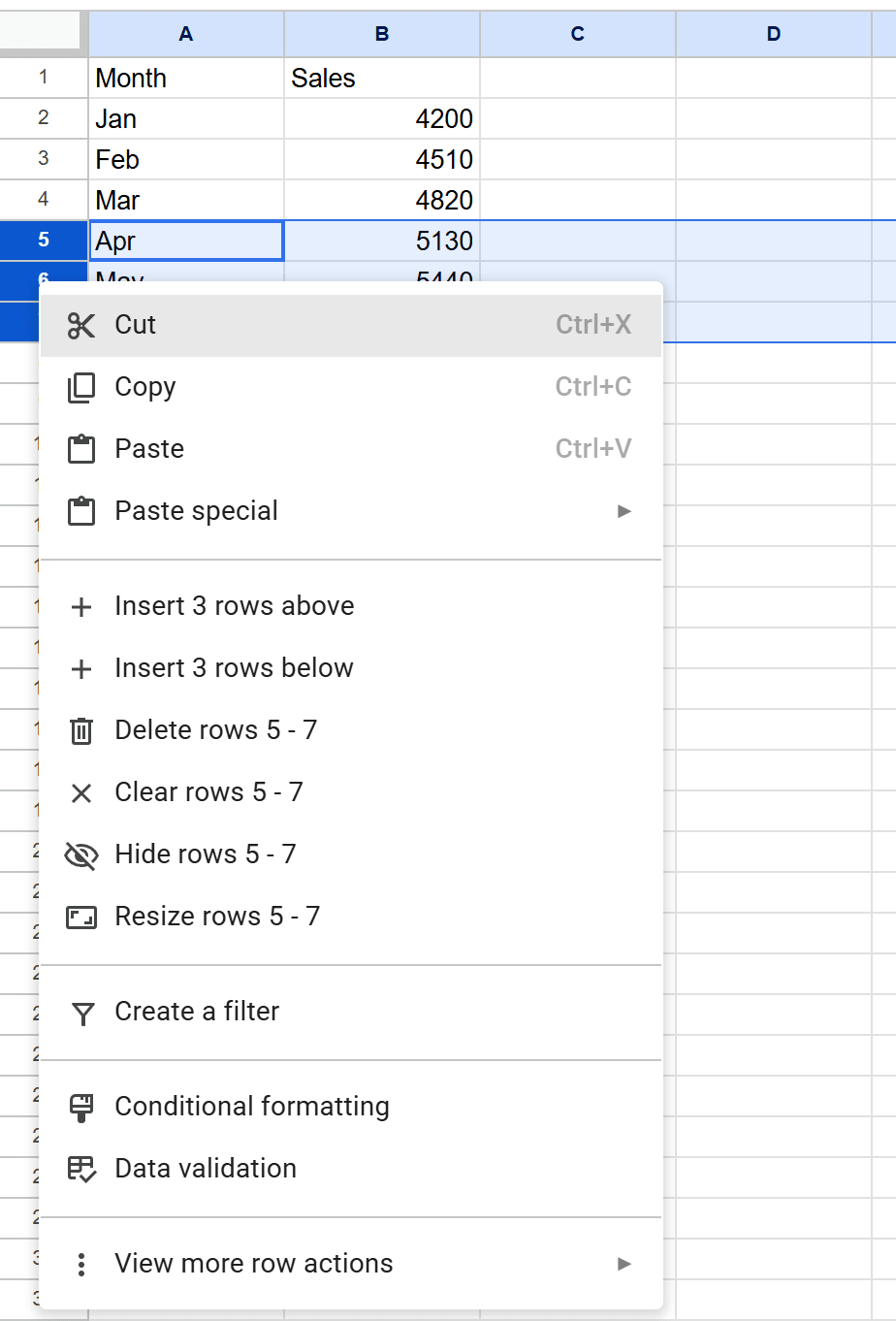
Click a row number to select the whole row. To select several rows next to each other, click the first row number and Shift-click the last. Here that’s rows 5 to 7.
2
Right-click and choose Hide
Right-click one of the selected row numbers. With one row selected the option reads Hide row. With several, it names the range: Hide rows 5 - 7.
3
Check the arrows
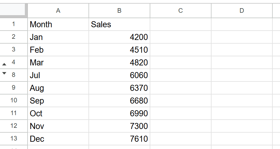
The rows disappear, and the row numbers skip from 4 to 8. Small arrows appear on the row numbers either side of the gap. That’s the only sign rows are hidden, so it’s easy to miss.
How to Hide Columns
Columns work the same way. Right-click a column letter and choose Hide column, or select several letters first. Arrows appear on the column letters on either side of the hidden ones.
How to Unhide Rows and Columns
- Click an arrow. Click either arrow next to the hidden rows or columns and they reappear.
- Use the shortcut. Select the rows on both sides of the hidden ones, for example rows 4 to 8, and press Ctrl+Shift+9. For columns, press Ctrl+Shift+0.
Keyboard Shortcuts
These are the shortcuts listed in Google Sheets’ own shortcut panel (Ctrl+/):
| Action | Shortcut |
|---|---|
| Hide rows | Ctrl+Alt+9 |
| Hide columns | Ctrl+Alt+0 |
| Unhide rows | Ctrl+Shift+9 |
| Unhide columns | Ctrl+Shift+0 |
| Group rows or columns | Alt+Shift+→ |
| Ungroup | Alt+Shift+← |
| Collapse a group | Alt+Shift+↑ |
| Expand a group | Alt+Shift+↓ |
Ctrl+9 and Ctrl+0 also hide rows and columns, but only if compatible spreadsheet shortcuts are turned on in the shortcut panel. More in the Google Sheets shortcuts cheat sheet.
Group Rows Instead of Hiding Them
Hidden rows are easy to lose track of. Grouping keeps the same rows collapsible, with a visible button anyone can click.
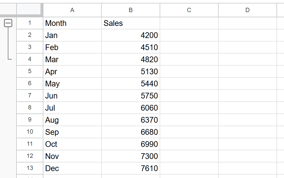
- Select the rows, for example rows 2 to 4 for January to March. Typing 2:4 in the Name Box at the top left selects them exactly.
- Press Alt+Shift+→, or go to View > Group > Group.
A bracket appears in the margin with a minus button. Click it to collapse the rows and a plus button replaces it.
Use grouping for anything a reader should be able to open: monthly detail under a quarterly total, or the working steps under a result. Use hiding for things nobody needs to see.
Do Formulas Include Hidden Rows?
Yes. Hiding a row doesn’t take it out of your formulas. In a test with twelve months of 100 each and three months hidden:
| Formula | Result | Hidden rows |
|---|---|---|
=SUM(B11:B22) | 1,200 | Included |
=SUBTOTAL(9,B11:B22) | 1,200 | Included |
=SUBTOTAL(109,B11:B22) | 900 | Skipped |
To total only the rows you can see, use SUBTOTAL with a function code of 101 to 111. 109 is SUM, 101 is AVERAGE, 103 is COUNTA. The codes 1 to 11 do the same math but include hidden rows.
Hide a Whole Sheet
To hide an entire tab, right-click it at the bottom of the screen and choose Hide sheet. To bring it back, go to View > Hidden sheets and pick it from the list.
Warning
Hiding isn’t security. Anyone who can edit the sheet can unhide rows, columns and tabs, and hidden data comes along in downloads and copies. To stop edits, use protected ranges. To keep data private, don’t share it.
Related Google Sheets Tutorials
- Freeze Rows and Columns - Keep headers on screen while you scroll
- Google Sheets Shortcuts - Every keyboard shortcut in one place
- Protect Sheets and Ranges - Stop people editing what they shouldn’t
- How to Sort and Alphabetize - Reorder rows without losing any
Frequently Asked Questions
How do I unhide rows in Google Sheets?
Click the small arrow on the row number above or below the hidden rows. You can also select the rows on both sides of the hidden ones and press Ctrl+Shift+9.
What is the shortcut to hide rows in Google Sheets?
Ctrl+Alt+9 hides the selected rows and Ctrl+Alt+0 hides the selected columns. Ctrl+Shift+9 and Ctrl+Shift+0 unhide them.
How do I hide columns in Google Sheets?
Right-click the column letter and choose Hide column, or select the column and press Ctrl+Alt+0. Arrows appear on the neighboring column letters so you can show it again.
What's the difference between hiding and grouping rows?
Hiding makes rows disappear with only small arrows to show they're gone. Grouping adds a plus or minus button in the margin, so anyone can collapse and expand the rows with one click. Group with Alt+Shift+Right arrow.
Can other people see rows I've hidden?
Anyone who can edit the sheet can unhide them, and hidden rows still show up in downloads and copies. Hiding tidies a view. It doesn't protect or secure data.
You've googled this formula before. Probably more than once.
The Bootcamp is a real Google Sheet that grades every formula the moment you press Enter. 193 exercises across 9 modules, the 10% of Sheets that does 90% of the work. One payment of $29.
Get It for $29 Get the Bootcamp for $2930-day refund. Reply to any email and you get your money back.
Not ready to pay? Try Basic Training free →