
Make the result range span several columns and one XLOOKUP returns them all: =XLOOKUP("SKU-103", A2:A6, B2:D6) returns the product’s name, category, and price in three cells. The extra values spill into the cells to the right, which must be empty or the formula returns #REF!.
intermediate 3 min read
XLOOKUP Return Multiple Columns in Google Sheets
Return several columns from one XLOOKUP in Google Sheets. How spilling works, fixing the #REF! blocked-spill error, and multi-column lookup patterns.
SB
Sheets Bootcamp
July 28, 2026
Table of Contents
Quick Answer
A record lookup usually wants more than one field: find the order, show the product, the date, and the amount. With VLOOKUP that means three formulas with three column indexes. XLOOKUP does it in one, because the result range is a real range and nothing says it has to be one column wide.
In This Guide
- One Formula, Several Columns
- How Spilling Works
- Fixing the #REF! Blocked Spill
- Building Record Cards and Tables
- What This Cannot Do
- Related Google Sheets Tutorials
One Formula, Several Columns
The inventory table:
| Product ID | Product Name | Category | Price |
|---|---|---|---|
| SKU-101 | Magnifying Glass | Optics | $24.99 |
| SKU-102 | Forensic Chemistry Set | Lab | $45.00 |
| SKU-103 | Pocket Watch | Accessories | $35.00 |
| SKU-104 | Field Binoculars | Optics | $65.00 |
| SKU-105 | Cipher Decoder | Accessories | $28.50 |
Everything about SKU-103 in one formula:
Formula
=XLOOKUP("SKU-103", A2:A6, B2:D6) The cell holding the formula shows “Pocket Watch”, the next cell to the right shows “Accessories”, and the one after that shows $35.00. One formula, three results.
How Spilling Works
XLOOKUP finds the matching row, then hands back that row’s slice of the result range: one value per column. The first value lands in the formula’s own cell, and the rest spill into the neighbors to the right, in order.
Only the first cell contains a formula. Click a spilled cell and the formula bar shows it is empty; its value is projected there by the formula to its left. Delete the formula and every spilled value disappears with it, which is exactly what you want: the record stays in sync as one unit.
The result range’s width decides the spill width. B2:C6 spills two cells, B2:D6 spills three. The lookup range stays one column either way; only the results widen.
Fixing the #REF! Blocked Spill
If any cell in the spill zone already holds data, the formula cannot expand, and instead of returning partial results it returns #REF!:
Formula
=XLOOKUP("SKU-103", A2:A6, B2:D6) With text sitting two cells to the right, that formula shows #REF! in its own cell and nothing spills. We verified the behavior directly: the same formula that returns three values with clear neighbors returns #REF! the moment one of those cells is occupied.
The fix is always the same: clear the cells to the right of the formula, as many as the result range is wide, minus one. If clearing is not an option because something lives there, either narrow the result range or move the formula.
Note
A #REF! from a blocked spill is not caught by the missing_value argument, which only handles the not-found case. If you see #REF!, the problem is space, not data.
Building Record Cards and Tables
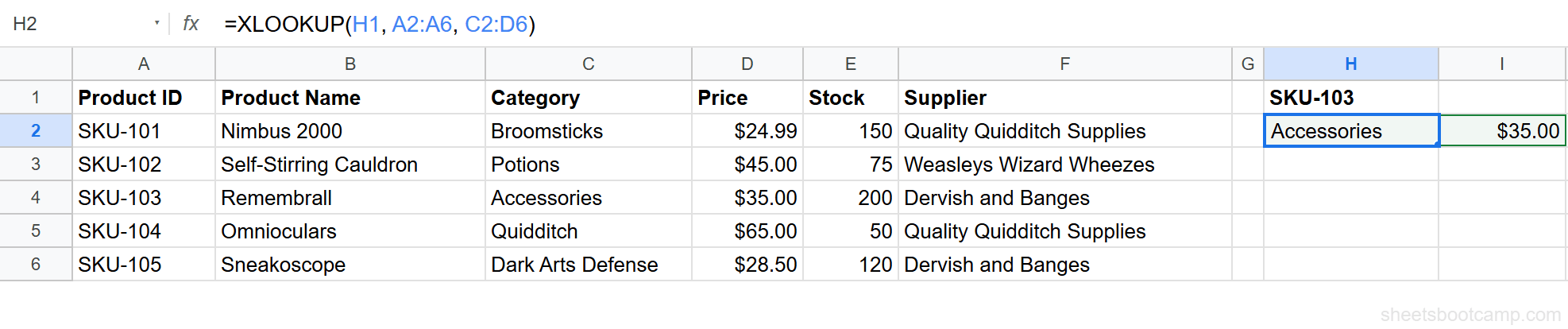
A record card. Put the search key in one cell (say H1), and one multi-column XLOOKUP beside it. Type a different ID into H1 and the whole record updates. This is the cleanest way to build a “look up an order” panel on a dashboard.
Formula
=XLOOKUP(H1, A2:A6, B2:D6, "ID not found") A joined table. Drag the formula down a column of keys, and each row spills its own results:
Formula
=XLOOKUP(G2, $A$2:$A$100, $B$2:$D$100, "") Lock the table ranges with $ so dragging moves only the search key. Every spill column must be empty all the way down. This pattern joins a table of IDs to their details in a single dragged formula, which with VLOOKUP would take one formula per field.
Tip
Give the spill columns real headers even though their cells hold no formulas. The headers document what lands where, and anyone editing the sheet learns not to type in the spill zone.
What This Cannot Do
The result range must be one contiguous block. To return columns B and D but not C, use two formulas, one per column. And XLOOKUP returns exactly one matching row per search: to get every row where a condition holds, reach for FILTER instead, which returns as many rows as match. XLOOKUP answers “which one,” FILTER answers “which ones.”
For the multi-condition version of “which one,” see XLOOKUP with multiple criteria: the boolean-array lookup range combines cleanly with a multi-column result range.
Related Google Sheets Tutorials
- XLOOKUP: The Complete Guide: The function end to end
- XLOOKUP Errors: #REF! and the rest of the family
- XLOOKUP with Multiple Criteria: Multi-condition record lookups
- FILTER Function: Return every matching row, not just one
- XLOOKUP Horizontal Lookups: Spilling downward from row-based lookups
Frequently Asked Questions
Can XLOOKUP return more than one column in Google Sheets?
Yes. Set the result_range to span several columns and one formula returns all of them: =XLOOKUP("SKU-103", A2:A6, B2:D6) returns the name, category, and price in three adjacent cells. The extra values spill to the right automatically.
Why does my multi-column XLOOKUP show #REF!?
The cells it needs to spill into are not empty. XLOOKUP writes the extra columns into the cells to the right of the formula; if any of them holds data, the whole formula returns #REF!. Clear those cells and the results appear.
Can XLOOKUP return multiple rows instead of columns?
XLOOKUP returns one matching row (or column, for horizontal lookups) per search. To return every row that matches a condition, use the FILTER function instead, which is built for exactly that.
Can I drag a multi-column XLOOKUP down a column?
Yes, the same way you drag any formula. Each row's formula spills its own results to the right, so leave all the spill columns empty. Lock the table ranges with $ so they do not shift as you drag.
How do I return non-adjacent columns with XLOOKUP?
A single result_range must be one contiguous block. For non-adjacent columns, use two XLOOKUP formulas, or wrap the row in a CHOOSECOLS-style selection. Two simple lookups side by side are usually the clearest option.
You've googled this formula before. Probably more than once.
The Bootcamp is a real Google Sheet that grades every formula the moment you press Enter. 193 exercises across 9 modules, the 10% of Sheets that does 90% of the work. One payment of $29.
Get It for $29 Get the Bootcamp for $2930-day refund. Reply to any email and you get your money back.
Not ready to pay? Try Basic Training free →