
XLOOKUP’s fourth argument replaces #N/A with anything you choose: =XLOOKUP(A2, B2:B50, C2:C50, "Not found") returns “Not found” when A2 is missing from the range. Unlike wrapping in IFERROR, it only catches the not-found case, so real formula mistakes still surface as errors.
beginner 3 min read
XLOOKUP If Not Found: The missing_value Argument
Handle missing lookups in Google Sheets with XLOOKUP's missing_value argument. Return text, zero, or a blank instead of #N/A, without wrapping in IFERROR.
SB
Sheets Bootcamp
July 28, 2026
Table of Contents
Quick Answer
Every lookup eventually searches for something that is not there. XLOOKUP is the first Google Sheets lookup function to treat that as a normal case instead of an error: the fourth argument, missing_value, is a built-in answer to “and what if it is missing?”
In This Guide
- The missing_value Argument
- Choosing a Fallback Value
- Why It Beats IFERROR
- Skipping It: The Double Comma
- What missing_value Does Not Catch
- Related Google Sheets Tutorials
The missing_value Argument
Formula
=XLOOKUP(search_key, lookup_range, result_range, [missing_value], [match_mode], [search_mode]) Without it, a failed lookup returns #N/A:
Formula
=XLOOKUP("SKU-999", A2:A6, D2:D6) With it, the same failure returns your value:
Formula
=XLOOKUP("SKU-999", A2:A6, D2:D6, "Not found") 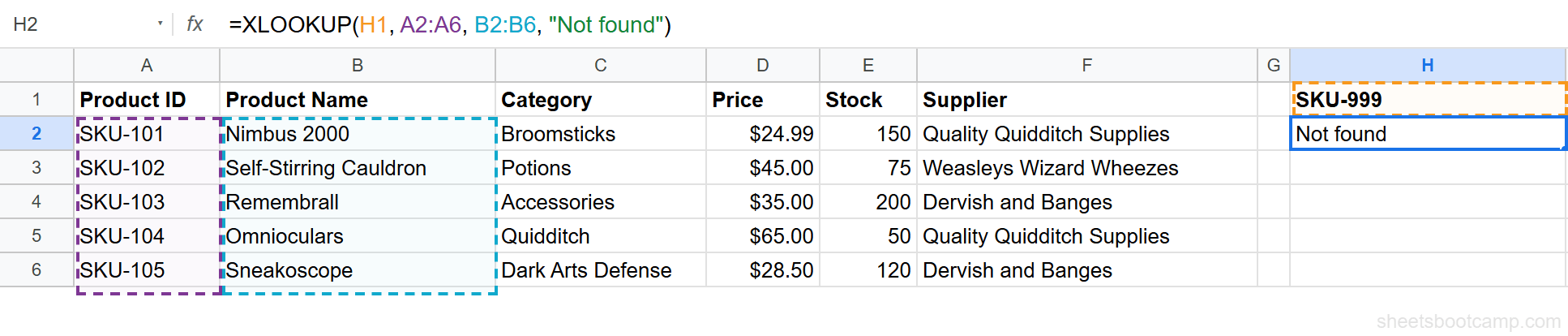
The fallback can be any value or even another formula: text, a number, an empty string, or a second lookup that tries a different table.
Choosing a Fallback Value
| Fallback | Formula | When to use |
|---|---|---|
| Text flag | =XLOOKUP(A2, B:B, C:C, “Not found”) | Human-read reports, obvious at a glance |
| Zero | =XLOOKUP(A2, B:B, C:C, 0) | Results feeding SUM, AVERAGE, or arithmetic |
| Blank | =XLOOKUP(A2, B:B, C:C, "") | Clean-looking dashboards |
| Second lookup | =XLOOKUP(A2, B:B, C:C, XLOOKUP(A2, Archive!B:B, Archive!C:C, “none”)) | Try the current table, then the archive |
The chained version in the last row is worth knowing: the fallback is itself an XLOOKUP, so a miss in the first table triggers a search of a second one. Only if both miss do you see “none”.
Tip
Match the fallback to what consumes the cell. A downstream SUM chokes on “Not found” but is fine with 0. A human scanning a report misses a 0 but spots “Not found” instantly.
Why It Beats IFERROR
Before XLOOKUP, the standard pattern wrapped the whole lookup:
Formula
=IFERROR(VLOOKUP(A2, B2:C50, 2, FALSE), "Not found") The problem: IFERROR catches every error, not just the not-found case. Delete a column so the range breaks, mistype the range, feed it text where a number belongs, and IFERROR hides the resulting #REF! or #VALUE! behind the same friendly “Not found”. The formula is broken and the sheet looks fine.
Missing_value is narrower. It answers only the question “what if the search key is not in the range?” Every other failure still shows its real error, which is exactly what you want: honest errors during building, friendly fallbacks in production.
Important
If you catch only one habit from this page: stop wrapping lookups in IFERROR by default. Use missing_value for the not-found case and let genuine mistakes stay visible. The narrower catch is covered in depth in IFERROR vs IFNA.
Skipping It: The Double Comma
Missing_value sits fourth, before match_mode and search_mode. To use those without a custom fallback, skip the slot with an empty argument:
Formula
=XLOOKUP(750, A2:A6, B2:B6, , -1) The two commas in a row mean “no missing_value, and match_mode is -1.” Skipped this way, a failed lookup still returns #N/A, which for a tier lookup is usually right: with match_mode -1, the only way to miss is a search key smaller than every bracket, and that deserves attention rather than a quiet fallback.
What missing_value Does Not Catch
Missing_value handles exactly one situation: no match found. It does not catch:
- #REF! from a blocked spill or a deleted range
- #VALUE! from array formulas that need ARRAYFORMULA
- #N/A from mismatched range sizes, where the lookup and result ranges have different lengths. This one is sneaky because it looks like a not-found result. If a lookup you know should succeed returns your fallback or #N/A, check the two ranges cover the same number of rows first.
The full troubleshooting list lives in XLOOKUP errors.
Related Google Sheets Tutorials
- XLOOKUP: The Complete Guide: All six parameters in one place
- XLOOKUP Errors: What each error means and how to fix it
- XLOOKUP Match Modes: The argument right after missing_value
- IFERROR vs IFNA: Error catching beyond lookups
- XLOOKUP vs VLOOKUP: Why VLOOKUP needs IFERROR and XLOOKUP does not
Frequently Asked Questions
How do I make XLOOKUP return a value instead of #N/A?
Set the fourth argument, missing_value. =XLOOKUP(A2, B2:B50, C2:C50, "Not found") returns the text Not found whenever A2 is not in the lookup range, with no IFERROR needed.
How do I make XLOOKUP return blank instead of #N/A?
Pass an empty string as the fourth argument: =XLOOKUP(A2, B2:B50, C2:C50, ""). The cell displays nothing when there is no match. Note that downstream formulas see an empty text value, not a truly empty cell.
Should I use XLOOKUP missing_value or IFERROR?
Use missing_value. It only catches the not-found case, while IFERROR swallows every error including real mistakes like a mistyped range. A broken formula wrapped in IFERROR shows your fallback text instead of telling you it is broken.
Why does XLOOKUP still show #N/A when I set missing_value?
Check the argument position. Missing_value is the fourth argument, before match_mode and search_mode. If you wrote the fallback in the wrong slot, it may be interpreted as a match mode instead. Also confirm the error is really #N/A: missing_value does not catch #REF! or #VALUE! errors.
What should missing_value be for numeric lookups?
Usually 0 for values you will sum or average, since text would break the math. But consider whether 0 is honest: a missing price is not a free product. For reports, a text flag like "missing" in a separate check column is often safer.
You've googled this formula before. Probably more than once.
The Bootcamp is a real Google Sheet that grades every formula the moment you press Enter. 193 exercises across 9 modules, the 10% of Sheets that does 90% of the work. One payment of $29.
Get It for $29 Get the Bootcamp for $2930-day refund. Reply to any email and you get your money back.
Not ready to pay? Try Basic Training free →