
To multiply in Google Sheets, use an asterisk: =B2*D2. To divide, use a forward slash: =B2/D2. With $250 in B2 and 5 in D2, =B2/D2 returns $50. The functions MULTIPLY, PRODUCT and DIVIDE do the same jobs, and a zero or blank divisor returns #DIV/0!.
beginner 3 min read
How to Multiply and Divide in Google Sheets
Multiply in Google Sheets with * or PRODUCT and divide with / or DIVIDE. Multiply a column by a number, fix #DIV/0!, and get a quotient and remainder.
SB
Sheets Bootcamp
September 30, 2026
Table of Contents
Quick Answer
Multiplying and dividing in Google Sheets work exactly like on a calculator, with two symbols to remember: * for multiply and / for divide. This page covers both, plus the functions that go with them, how to apply a formula to a whole column, and how to deal with the #DIV/0! error.
The examples use a small order sheet with each customer’s order Total and number of Items.
How to Multiply in Google Sheets
Type an equals sign, the first value, an asterisk, and the second value:
Formula
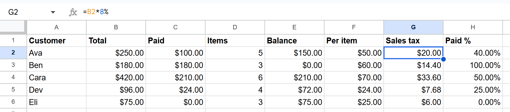
=B2*D2 Multiplication works with cells, numbers, or both. To work out 8% sales tax on each order total:
Formula
=B2*8% Ava’s $250 order has $20 of tax. Fill the formula down and each row calculates its own.
The MULTIPLY and PRODUCT functions
MULTIPLY takes two values and multiplies them: =MULTIPLY(B2,D2) returns the same result as =B2*D2.
PRODUCT multiplies everything in a range together:
Formula
=PRODUCT(D2:D4) With 2, 3 and 4 in D2:D4, it returns 24. PRODUCT skips text inside a range: add a cell that says “n/a” to the range and the answer is still 24. The asterisk doesn’t: =B2*D5, where D5 says “n/a”, returns #VALUE!.
Multiply a column by one number
Put the number in its own cell, say a tax rate in E1, and lock it with dollar signs:
Formula
=B2*$E$1 Fill it down and every row multiplies by E1. Without the dollar signs, the reference would shift to E2, E3 and so on as you fill down. Absolute and relative references explains why.
Multiply two columns row by row
To multiply every price by its quantity without filling down, use ARRAYFORMULA:
Formula
=ARRAYFORMULA(B2:B4*D2:D4) With prices of 100, 60 and 40 and quantities of 2, 3 and 4, it spills 200, 180 and 160 down the column. To multiply the columns and add the results in one step, use =SUMPRODUCT(B2:B4,D2:D4), which returns 540. See the ARRAYFORMULA guide for more.
How to Divide in Google Sheets
Use a forward slash:
Formula
=B2/D2 To find the average price per item on each order, divide the Total by the Items. Ava’s $250 across 5 items is $50 per item.
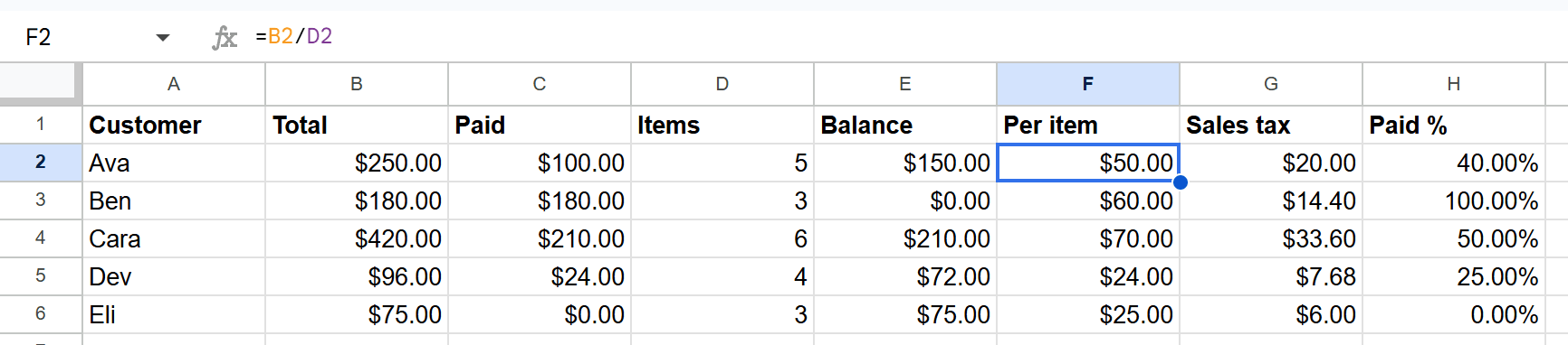
The DIVIDE function does the same thing: =DIVIDE(B2,D2) also returns $50.
Quotient and remainder
When you want the whole-number result of a division and what’s left over, use QUOTIENT and MOD:
| Formula | Result | What it gives you |
|---|---|---|
=60/7 | 8.57… | The full answer |
=QUOTIENT(60,7) | 8 | The whole-number part only |
=MOD(60,7) | 4 | The remainder |
Handy for things like splitting 60 items into boxes of 7: 8 full boxes, 4 items left over.
How to Fix #DIV/0!
#DIV/0! means you divided by zero. In Google Sheets that happens two ways:
- The divisor is 0.
- The divisor is a blank cell. Blank counts as zero, so =B2/C5 with C5 empty returns #DIV/0! too.
To show something friendlier, wrap the division in IFERROR:
Formula
=IFERROR(B2/D2, 0) When D2 is zero, that returns 0 instead of an error. You can return a blank with "" or a word like "n/a" instead.
Warning
IFERROR hides every error, not just #DIV/0!. If a typo breaks the formula, IFERROR hides that too. Use it once the formula already works.
Related Google Sheets Tutorials
- How to Subtract in Google Sheets - Minus sign formulas and the MINUS function
- Percentages in Google Sheets - Percent of total, change, and discounts
- IFERROR - Replace errors with a value of your choice
- ARRAYFORMULA - Apply one formula to a whole column
Frequently Asked Questions
How do you multiply in Google Sheets?
Use an asterisk: =B2*D2 multiplies the values in B2 and D2. With 100 and 2, it returns 200. To multiply every number in a range together, use =PRODUCT(D2:D4).
How do you divide in Google Sheets?
Use a forward slash: =B2/D2. With 250 and 5, it returns 50. The DIVIDE function, =DIVIDE(B2,D2), gives the same result.
Why does my division formula show #DIV/0!?
The divisor is zero or blank. Both =B2/0 and dividing by an empty cell return #DIV/0!. Wrap the formula in IFERROR to show something else: =IFERROR(B2/D2,0).
How do I multiply a whole column by one number?
Put the number in a cell, for example E1, and use =B2*$E$1 in the first row, then fill down. The dollar signs keep every row pointing at E1.
How do I get the remainder when dividing?
Use MOD. =MOD(60,7) returns 4. QUOTIENT gives the whole-number part: =QUOTIENT(60,7) returns 8.
You've googled this formula before. Probably more than once.
The Bootcamp is a real Google Sheet that grades every formula the moment you press Enter. 193 exercises across 9 modules, the 10% of Sheets that does 90% of the work. One payment of $29.
Get It for $29 Get the Bootcamp for $2930-day refund. Reply to any email and you get your money back.
Not ready to pay? Try Basic Training free →