
To subtract in Google Sheets, type an equals sign, the first cell, a minus sign, and the second cell: =B2-C2. With $250 in B2 and $100 in C2, it returns $150. Google Sheets has no SUBTRACT function, but =MINUS(B2,C2) does the same thing for two values.
beginner 3 min read
How to Subtract in Google Sheets (Formula and MINUS)
Subtract in Google Sheets with a minus sign formula like =B2-C2 or the MINUS function. Subtract columns, dates, percentages and whole ranges, with fixes for errors.
SB
Sheets Bootcamp
September 30, 2026
Table of Contents
Quick Answer
Subtraction in Google Sheets is a formula with a minus sign. There’s no button for it and no SUBTRACT function to look up. Once you have the one formula, the rest of this page is about applying it: to a whole column, to totals, to dates, to percentages, and to the errors that show up along the way.
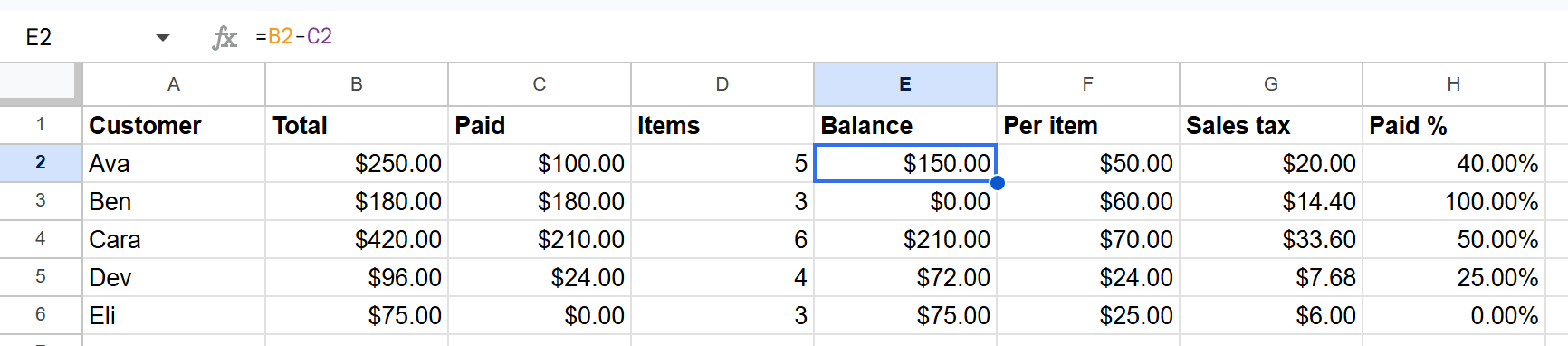
The examples use a small order sheet: each customer’s order Total, how much they’ve Paid, and the Balance still owed.
How to Subtract Two Cells
1
Click the result cell
Click the empty cell where the answer belongs. Here that’s E2, the first Balance cell.
2
Type the formula and press Enter
Type =B2-C2 and press Enter. Ava’s total of $250 minus the $100 she’s paid leaves a balance of $150.
3
Fill the formula down the column
Click E2, then drag the small blue square in its bottom-right corner down to E6. Each row subtracts its own cells: E3 becomes =B3-C3, E4 becomes =B4-C4, and so on.
Tip
Always point the formula at cells, not typed numbers. =B2-C2 updates by itself when Ava pays more. =250-100 doesn’t.
The MINUS Function
Google Sheets has a function for subtraction, but it’s called MINUS, not SUBTRACT:
Formula
=MINUS(B2, C2) It returns the same $150. The catch is that MINUS takes exactly two values. Give it a range, like =MINUS(B2:B3,1), and it returns #VALUE!. For three or more values, use minus signs: =B2-C2-D2.
How to Subtract a Whole Column
There are two different things “subtract a column” can mean.
Row by row. Put =B2-C2 in the first row and fill it down, as above. Or do the whole column with one formula:
Formula
=ARRAYFORMULA(B2:B6-C2:C6) That returns one balance per row, starting in the cell you typed it in and spilling down. Leave the cells below it empty, or it can’t spill.
Total minus total. To subtract one column’s total from another’s, subtract two SUMs:
Formula
=SUM(B2:B6)-SUM(C2:C6) Subtract a Range from a Single Number
To take several cells away from one number, subtract their SUM. If a budget of $100 sits in B2 and three expenses sit in C2:C4:
Formula
=B2-SUM(C2:C4) With expenses of $35, $25 and $30, the result is $10. This is cleaner than =B2-C2-C3-C4 and doesn’t break when you add a row to the range.
Subtract a Percentage
To take 10% off a price in B2, multiply by 1 minus the percentage:
Formula
=B2*(1-10%) A $100 price becomes $90. Writing =B2-10% instead subtracts 0.1, not 10% of the price, so the answer comes out as $99.90. More on this in percentages in Google Sheets.
Subtract Dates
Dates in Google Sheets are numbers, one per day, so subtracting two dates returns the days between them:
Formula
=DATE(2026,3,15)-DATE(2026,3,1) That returns 14. With real dates in cells, it’s just =B2-A2. If the result shows up as a date instead of a number, change the cell’s format to Number. For months or years between two dates, use DATEDIF, and for adding or subtracting days from a date, see add or subtract days, months and years.
Subtraction Errors and Surprises
#VALUE! One of the cells holds text. =A2-1, where A2 is the word “Notebook”, returns #VALUE!. Check for numbers that were pasted in as text, which often sit on the left side of the cell.
A negative result. That’s correct math, not an error. =C2-B2 with $35 and $100 returns -65. Swap the cells if you wanted it the other way around.
A blank cell. Blank cells count as zero, so =B5-C5 with $20 and an empty C5 returns $20. That’s usually what you want, but it can hide a missing value.
Related Google Sheets Tutorials
- Multiply and Divide in Google Sheets - The other arithmetic formulas
- Percentages in Google Sheets - Percent of total, percent change, and discounts
- SUM Function - Add up a column before you subtract it
- Absolute and Relative References - Keep a reference fixed when you fill down
Frequently Asked Questions
What is the subtraction formula in Google Sheets?
Type an equals sign, the first value, a minus sign, and the second value, for example =B2-C2. With $250 in B2 and $100 in C2, it returns $150.
Is there a SUBTRACT function in Google Sheets?
No. The subtraction function is MINUS, for example =MINUS(B2,C2). It takes exactly two values, so for anything more use the minus sign, like =B2-C2-D2.
How do I subtract a whole column in Google Sheets?
Subtract the totals: =SUM(B2:B6)-SUM(C2:C6). To subtract row by row, put =B2-C2 in the first row and drag it down, or use =ARRAYFORMULA(B2:B6-C2:C6) to fill the whole column at once.
How do I subtract dates in Google Sheets?
Subtract the earlier date from the later one. =DATE(2026,3,15)-DATE(2026,3,1) returns 14, the number of days between them.
Why does my subtraction formula show #VALUE!?
One of the cells holds text, not a number. Subtracting 1 from a cell containing the word Notebook returns #VALUE!. Blank cells don't cause the error: they count as zero.
You've googled this formula before. Probably more than once.
The Bootcamp is a real Google Sheet that grades every formula the moment you press Enter. 193 exercises across 9 modules, the 10% of Sheets that does 90% of the work. One payment of $29.
Get It for $29 Get the Bootcamp for $2930-day refund. Reply to any email and you get your money back.
Not ready to pay? Try Basic Training free →